The next model in the FluxArchitectures repository is the Temporal Pattern Attention LSTM network based on the paper “Temporal Pattern Attention for Multivariate Time Series Forecasting” by Shih et. al.. It claims to have a better performance than the previously implemented LSTNet, with the additional advantage that an attention mechanism automatically tries to determine important parts of the time series, instead of introducing parameters that need to be optimized by the user.
Model Architecture
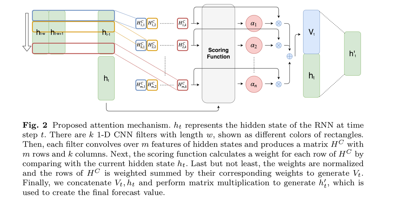
Image from Shih et. al., “Temporal Pattern Attention for Multivariate Time Series Forecasting”, ArXiv, 2019.
The neural net consists of the following elements: The first part consists of an embedding and stacked LSTM layer made up of the following parts:
- A
Denseembedding layer for the input data. - A
StackedLSTMlayer for the transformed input data.
The temporal attention mechanism consist of
- A
Denselayer that transforms the hidden state of the last LSTM layer in theStackedLSTM. - A convolutional layer operating on the pooled output of the previous layer, estimating the importance of the different datapoints.
- A
Denselayer operating on the LSTM hidden state and the output of the attention mechanism.
A final Dense layer is used to calculate the output of the network.
The code is based on a PyTorch implementation by Jing Wang of the same model with slight adjustments.
We define a struct to hold all layers and some metadata:
mutable struct TPALSTMCell
    # Prediction layers
    embedding::A
    output::B
    lstm::C
    # Attention layers
    attention_linear1::D
    attention_linear2::E
    attention_conv::F
	# Metadata ...
end
These layers are initialized as follows:
function TPALSTM(in, hiddensize, poollength, layers=1, filternum=32, filtersize=1)
	embedding = Dense(in, hiddensize, Flux.relu)
    output = Dense(hiddensize, 1)
    lstm = StackedLSTM(hiddensize, hiddensize, hiddensize, layers)
    attention_linear1 = Dense(hiddensize, filternum)
    attention_linear2 = Dense(hiddensize + filternum, hiddensize)
    attention_conv = Conv((filtersize, poollength - 1), 1 => filternum)
    return TPALSTMCell(...)
end
We use the same input data format as for the previous LSTnet layer, i.e. “Number of input features x Number of pooled timesteps x 1 x Number of data points”. The StackedLSTM layer is described later - it is basically a number of LSTM layers, where the hidden state of one layer gets fed to the next layer as input.
The model output is obtained by the following function:
function (m::TPALSTMCell)(x)
    inp = dropdims(x, dims=3)  # num_features x poollength x batchsize
    H_raw = _TPALSTM_gethidden(inp, m)
	H = Flux.relu.(H_raw)  # hiddensize x (poollength - 1) x batchsize
    x = inp[:,end,:]  # num_features x batchsize
    xconcat = m.embedding(x)  # hiddensize x batchsize
    _ = m.lstm(xconcat)
    h_last = m.lstm.chain[end].state[1]  # hiddensize x batchsize
    ht = _TPALSTM_attention(H, h_last, m)  # hiddensize x batchsize
    return m.output(ht)  # 1 x batchsize
end
The following calculations are performed:
- Drop the singleton dimension of the input data.
- Get the hidden state from feeding a section of past input data to the stacked LSTM network.
- Obtain the hidden state for the current input data.
- Transform this hidden state by the attention mechanism.
- Obtain the final output.
Step 2 and 5 are described in the following subsections.
Obtaining the hidden states
This function basically runs through the pooled data, feeding it to the LSTM part of the network. In order to be able to collect the outputs, we use a Zygote.Buffer to store the results and return a copy to get back to normal arrays.
function _TPALSTM_gethidden(inp, m::TPALSTMCell)
    batchsize = size(inp,3)
    H = Flux.Zygote.Buffer(Array{Float32}(undef, m.hiddensize, m.poollength-1, batchsize))
    for t in 1:m.poollength-1
        x = inp[:,t,:]
        xconcat = m.embedding(x)
        _ = m.lstm(xconcat)
        hiddenstate = m.lstm.chain[end].state[1]
        H[:,t,:] = hiddenstate
    end
    return copy(H)
end
Attention mechanism
The attention mechanism is contained in the function
function _TPALSTM_attention(H, h_last, m::TPALSTMCell)
    H_u = Flux.unsqueeze(H, 3)  # hiddensize x (poollength - 1) x 1 x batchsize
    conv_vecs = Flux.relu.(dropdims(m.attention_conv(H_u), dims=2))  # (hiddensize - filtersize + 1) x filternum x batchsize

    w = m.attention_linear1(h_last) |>  # filternum x batchsize
        a -> Flux.unsqueeze(a, 1) |>  # 1 x filternum x batchsize
        a -> repeat(a, inner=(m.attention_features_size,1,1))  # (hiddensize - filtersize + 1) x filternum x batchsize
    alpha = Flux.sigmoid.(sum(conv_vecs.*w, dims=2))  # (hiddensize - filtersize + 1) x 1 x batchsize
    v = repeat(alpha, inner=(1,m.filternum,1)) |>  # (hiddensize - filtersize + 1) x filternum x batchsize
        a -> dropdims(sum(a.*conv_vecs, dims=1), dims=1)  # filternum x batchsize

    concat = cat(h_last, v, dims=1)  # (filternum + hiddensize) x batchsize
    return m.attention_linear2(concat)  # hiddensize x batchsize
end
It consists of the following steps:
- We make sure that the matrix of pooled hidden states
Hhas the right shape for a convolutional network by adding a third dimension of size one (making it the same size as the original input data). - The
Convlayer is applied, followed by areluactivation function. - The transformed current hidden state of the LSTM part is multiplied with the output of the convolutional net. A
sigmoidactivation function gives attention weightsalpha. - The output of the convolutional net is weighted by the attention weights and concatenated with the current hidden state of the LSTM part.
- A
Denselayer reduces the size of the concatenated vector.
Stacked LSTM
The stacked version of a number of LSTM cells is obtained by feeding the hidden state of one cell as input to the next one. Flux.jl’s standard setup only allows feeding the output of one cell as the new input, thus we adjust some of the internals:
- Management of hidden states in
Fluxis done by theRecurstructure, which returns the output of a recurrent layer. We use a similarHiddenRecurstructure instead which returns the hidden state.
mutable struct HiddenRecur{T}
  cell::T
  init
  state
end

function (m::HiddenRecur)(xs...)
  h, y = m.cell(m.state, xs...)
  m.state = h
  return h[1]  # return hidden state of LSTM
end
- The
StackedLSTM-function chains everything together depending on the number of layers. (One layer corresponds to a standardLSTMcell.)
mutable struct StackedLSTMCell{A}
	chain::A
end

function StackedLSTM(in, out, hiddensize, layers::Integer)
	if layers == 1  # normal LSTM cell
		chain = Chain(LSTM(in, out))
	elseif layers == 2
		chain = Chain(HiddenRecur(Flux.LSTMCell(in, hiddensize)),
					LSTM(hiddensize, out))
	else
		chain_vec=[HiddenRecur(Flux.LSTMCell(in, hiddensize))]
		for i=1:layers-2
			push!(chain_vec, HiddenRecur(Flux.LSTMCell(hiddensize, hiddensize)))
		end
		chain = Chain(chain_vec..., LSTM(hiddensize, out; init = init))
	end
	return StackedLSTMCell(chain)
end

function (m::StackedLSTMCell)(x)
	return m.chain(x)
end