The next model in the FluxArchitectures repository is the “Dual-Stage Attention-Based Recurrent Neural Network for Time Series Prediction”, based on the paper by Qin et. al., 2017. It claims to have a better performance than the previously implemented LSTNet, with the additional advantage that an attention mechanism automatically tries to determine important parts of the time series, instead of introducing parameters that need to be optimized by the user.
Model Architecture
The neural network has a rather complex structure. Starting with an encoder-decoder structure, it consists of two units, one called the input attention mechanism, and a temporal attention mechanism.
-
The input attention mechanism feeds the input data to a LSTM network. In subsequent calculations, only its hidden state is used, where additional network layers try to estimate the importance of different hidden variables.
-
The temporal attention mechanism takes the hidden state of the encoder network and combines it with the hidden state of another LSTM decoder. Additional network layers try again to estimate the importance of the hidden variables of the encoder and decoder combined.
-
Linear layers combine the output of different layers to the final time series prediction.
Our implementation follows the one for PyTorch. We start out by creating a struct to hold all the necessary elements:
mutable struct DARNNCell{A, B, C, D, E, F, W, X, Y, Z}
  # Encoder part
	encoder_lstm::A
	encoder_attn::B
  # Decoder part
	decoder_lstm::C
	decoder_attn::D
	decoder_fc::E
	decoder_fc_final::F
  # Index for original data etc
	encodersize::W
	decodersize::X
	orig_idx::Y
	poollength::Z
end
In addition to the layers we need for constructing the DA-RNN network, we also store some metadata that are needed for the calculations: The size of the encoder and decoder network, the index orig_idx describing where in the input data the original time series can be found, and the number of time steps that the input data was pooled (corresponding to T in the following picture).
The constructor initializes all layers with their correct size:
function DARNN(inp::Integer, encodersize::Integer, decodersize::Integer, poollength::Integer, orig_idx::Integer)
	# Encoder part
	encoder_lstm = LSTM(inp, encodersize)
	encoder_attn = Chain(Dense(2*encodersize + poollength, poollength),
	                    a -> tanh.(a),
	                    Dense(poollength,1)
	# Decoder part
	decoder_lstm = LSTM(1, decodersize)
	decoder_attn = Chain(Dense(2*decodersize + encodersize, encodersize),
	                    a -> tanh.(a),
	                    Dense(encodersize, 1))
	decoder_fc = Dense(encodersize + 1, 1)
	decoder_fc_final = Dense(decodersize + encodersize, 1)

	return DARNNCell(encoder_lstm, encoder_attn, decoder_lstm, decoder_attn, decoder_fc,
	 		  decoder_fc_final, encodersize, decodersize, orig_idx, poollength)
end
Encoder network
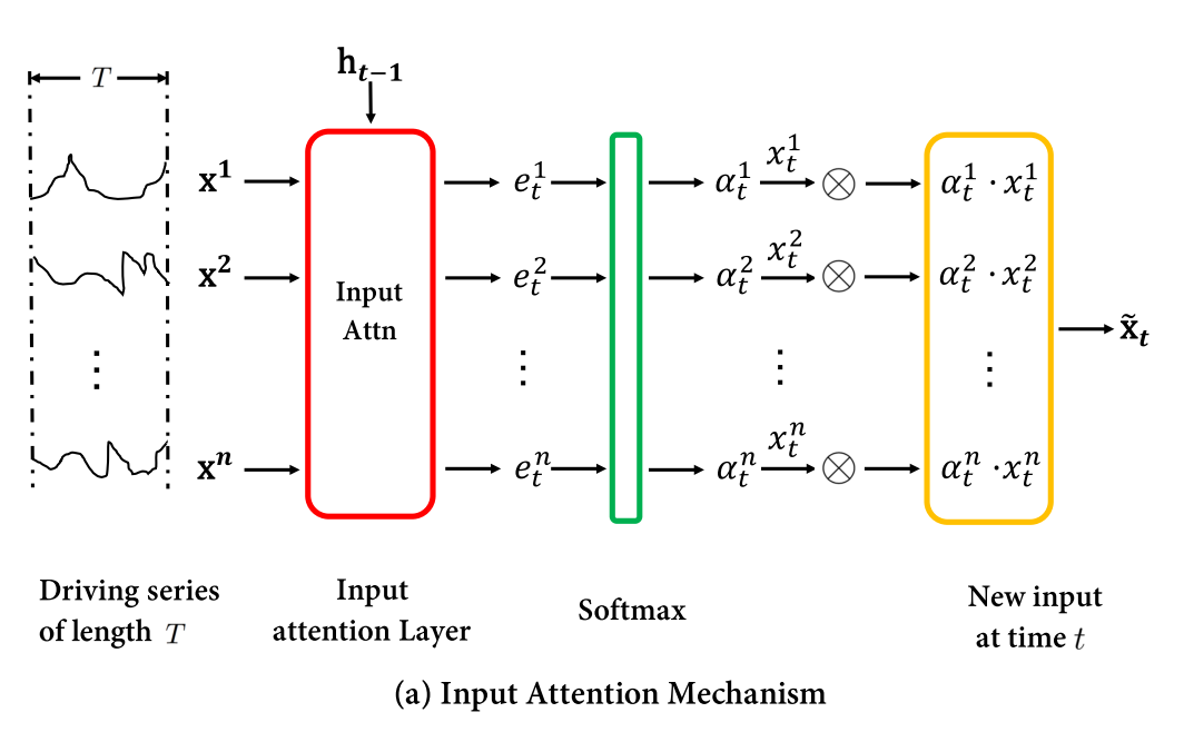
Image from Qin et. al., “Dual-Stage Attention-Based Recurrent Neural Network for Time Series Prediction”, ArXiv, 2017.
We use the same input data format as for the previous LSTnet layer, i.e. “Number of input features x Number of pooled timesteps x 1 x Number of data points”. Before feeding the data to the encoder, we drop the singleton dimension: input_data = dropdims(x; dims=3).
The encoder loops over the pooled timesteps to perform a scaling of the input data: It extracts the hidden state and cell state of the encoder LSTM layer, concatenates it with the input data and feeds it to the attention network. Using a softmax function, we obtain the scaling for the input data for timestep t, which is fed to the LSTM network. In the following code, we indicate the equation numbers from the paper cited in the introduction.
for t in 1:m.poollength
  hidden = m.encoder_lstm.state[1]
  cell = m.encoder_lstm.state[2]

	# Eq. (8)
  x = cat(repeat(hidden, inner=(1,1,size(input_data,1))),
          repeat(cell, inner=(1,1,size(input_data,1))),
          permutedims(input_data,[2,3,1]), dims=1) |>  # (2*encodersize + poollength) x datapoints x features
			a -> reshape(a, (:, size(input_data,1)*size(input_data,3))) |>  # (2*encodersize + poollength) x (features * datapoints)
      m.encoder_attn  # features * datapoints

	# Eq. (9)
	attn_weights = Flux.softmax( reshape(x, (size(input_data,1), size(input_data,3))))  # features x datapoints
	# Eq. (10)
	weighted_input = attn_weights .* input_data[:,t,:]  # features x datapoints
	# Eq. (11)
	_ = m.encoder_lstm(weighted_input)

  input_encoded[:,t,:] = Flux.unsqueeze(m.encoder_lstm.state[1],2)  # features x 1 x datapoints
end
In order to make this code trainable by Flux, we wrap the input_encoded into a Zygote.Buffer structure, and return copy(input_encoded).
Decoder Network
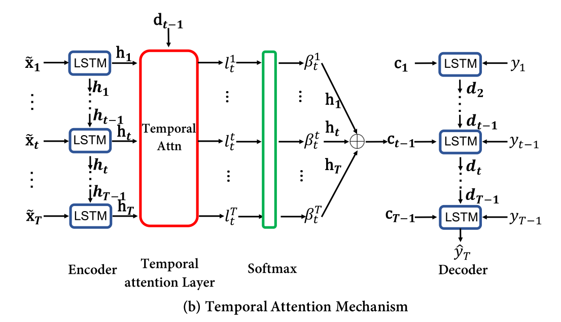
Image from Qin et. al., “Dual-Stage Attention-Based Recurrent Neural Network for Time Series Prediction”, ArXiv, 2017.
The decoder operates on input_encoded from the encoder, i.e. a collection of hidden states of the encoder LSTM network. It also loops over the pooled timesteps to calculate an “attention weight” to find relevant encoder hidden states and to calculate a “context vector” as a weighted sum of hidden states.
for t in 1:m.poollength
	# Extract hidden state and cell state from decoder
	hidden = m.decoder_lstm.state[1]
  cell = m.decoder_lstm.state[2]

	# Eq. (12) - (13)
	x = cat(permutedims(repeat(hidden, inner=(1,1,m.poollength)), [1,3,2]),
          permutedims(repeat(cell, inner=(1,1,m.poollength)), [1,3,2]),
          input_encoded, dims=1) |>  # (2*decodersize + encodersize) x poollength x datapoints
      a -> reshape(a, (2*m.decodersize + m.encodersize,:)) |>  #  (2*decodersize + encodersize) x (poollength * datapoints)
			m.decoder_attn |>  # poollength * datapoints
			a -> Flux.softmax(reshape(a, (m.poollength,:)))  # poollength x datapoints

	# Eq. (14)
	context = dropdims(NNlib.batched_mul(input_encoded, Flux.unsqueeze(x,2)), dims=2)  # encodersize x datapoints
	# Eq. (15)
	ỹ = m.decoder_fc(cat(context, input_data[m.orig_idx,t,:]', dims=1))  # 1 x datapoints
	# Eq. (16)
	_ = m.decoder_lstm(ỹ)
end
The decoder returns the context vector context of the last timestep.
Final Output
The final model output is obtained by feeding the encoder output to the decoder, and calling the final Dense layer on the concatenation of the decoder hidden state and the context vector:
function (m::DARNNCell)(x)
	# Initialization code missing...

	input_data = dropdims(x; dims=3)
	input_encoded = darnn_encoder(m, input_data)
	context = darnn_decoder(m, input_encoded, input_data)
	# Eq. (22)
	return m.decoder_fc_final( cat(m.decoder_lstm.state[1], context, dims=1))
end
Helper functions
To make sure that Flux knows which parameters to train, and how to reset the model, we define
Flux.trainable(m::DARNNCell) = (m.encoder_lstm, m.encoder_attn, m.decoder_lstm,
    m.decoder_attn, m.decoder_fc, m.decoder_fc_final)
Flux.reset!(m::DARNNCell) = Flux.reset!.((m.encoder_lstm, m.decoder_lstm))
When the DA-RNN network is reset, the number of hidden states in the LSTM units does not have the desired size. To initialize them, we feed input data of the right size manually to those layers:
function darnn_init(m::DARNNCell,x)
	m.encoder_lstm(x[:,1,1,:])
	m.decoder_lstm(x[m.orig_idx,1,1,:]')
	return nothing
end
Flux.Zygote.@nograd darnn_init