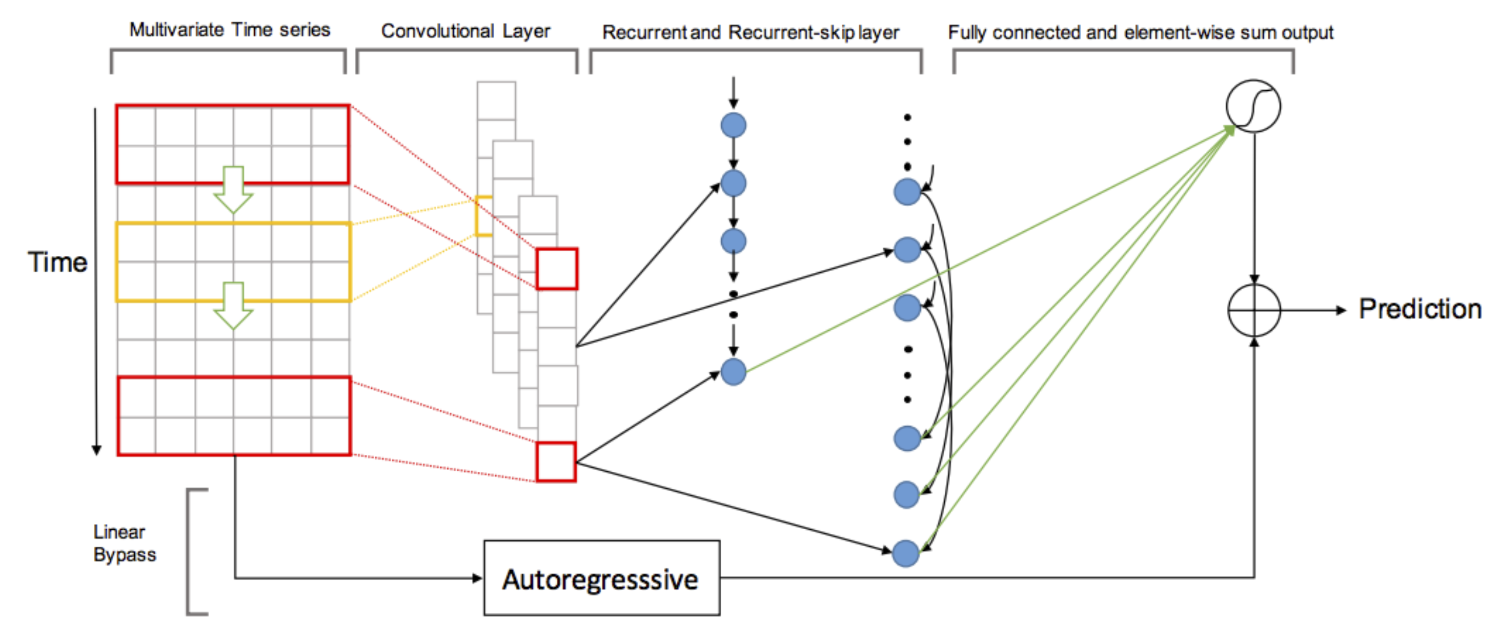
The first model in the FluxArchitectures repository is the “Long- and Short-term Time-series network” described by Lai et al., 2017.
Model Architecture

Image from Lai et al, “Long- and Short-term Time-series network”, ArXiv 2017.
The neural net consists of the following elements:
- A convolutional layer than operates on some window of the time series.
- Two recurrent layers: A
GRUcell withreluactivation function, and aSkipGRUcell similar to the previousGRUcell, with the difference that the hidden state is taken from a specific amount of timesteps back in time. Both theGRUand theSkipGRUlayer take their input from the convolutional layer. - A dense layer that operates on the concatenated output of the previous two layers.
- An autoregressive layer operating on the input data itself, being added to the output of the dense layer.
The Convolutional Layer
We use the standard Flux convolutional layer. Stemming from an image analysis background, it expects the input data to be in the “width, height, channels, batch size” order. For our application, we pool some window of the time series of input features together, giving
-
width: The number of input features.
-
height: The number of timesteps we pool together.
-
channels: We are only using one channel.
-
batch size: The number of convolutional layers
convlayersizewe would like to have in our model.
This gives
Conv((in, poolsize), 1 => convlayersize, σ)
Recurrent Layers
Flux has a GRU layer available, however with a different (fixed) activation function.1 Therefore we alter the code slightly to obtain our ReluGRU part of the model.
mutable struct ReluGRUCell{A,V}
  Wi::A
  Wh::A
  b::V
  h::V
end

ReluGRUCell(in, out; init = Flux.glorot_uniform) =
  ReluGRUCell(init(out*3, in), init(out*3, out),
          init(out*3), zeros(Float32, out))

function (m::ReluGRUCell)(h, x)
  b, o = m.b, size(h, 1)
  gx, gh = m.Wi*x, m.Wh*h
  r = σ.(Flux.gate(gx, o, 1) .+ Flux.gate(gh, o, 1) .+ Flux.gate(b, o, 1))
  z = σ.(Flux.gate(gx, o, 2) .+ Flux.gate(gh, o, 2) .+ Flux.gate(b, o, 2))
  h̃ = relu.(Flux.gate(gx, o, 3) .+ r .* Flux.gate(gh, o, 3) .+ Flux.gate(b, o, 3))
  h′ = (1 .- z).*h̃ .+ z.*h
  return h′, h′
end

Flux.hidden(m::ReluGRUCell) = m.h
Flux.@functor ReluGRUCell

"""
    ReluGRU(in::Integer, out::Integer)

Gated Recurrent Unit layer with `relu` as activation function.
"""
ReluGRU(a...; ka...) = Flux.Recur(ReluGRUCell(a...; ka...))
This is more or less a direct copy from the Flux code, only changing the activation function.
To get access to the hidden state of a ReluGRUCell from prior timepoints, we alter the gate function:
skipgate(h, n, p) = (1:h) .+ h*(n-1)
skipgate(x::AbstractVector, h, n, p) = x[skipgate(h,n,p)]
skipgate(x::AbstractMatrix, h, n, p) = x[skipgate(h,n,p),circshift(1:size(x,2),-p)]
With this, we can adapt the ReluGRU cell, add the skip-length parameter p to construct the SkipGRU part
mutable struct SkipGRUCell{N,A,V}
  p::N
  Wi::A
  Wh::A
  b::V
  h::V
end

SkipGRUCell(in, out, p; init = Flux.glorot_uniform) =
  SkipGRUCell(p, init(out*3, in), init(out*3, out),
          init(out*3), zeros(Float32, out))

function (m::SkipGRUCell)(h, x)
  b, o = m.b, size(h, 1)
  gx, gh = m.Wi*x, m.Wh*h
  p = m.p
  r = σ.(Flux.gate(gx, o, 1) .+ skipgate(gh, o, 1, p) .+ Flux.gate(b, o, 1))
  z = σ.(Flux.gate(gx, o, 2) .+ skipgate(gh, o, 2, p) .+ Flux.gate(b, o, 2))
  h̃ = relu.(Flux.gate(gx, o, 3) .+ r .* skipgate(gh, o, 3, p) .+ Flux.gate(b, o, 3))
  h′ = (1 .- z).*h̃ .+ z.*h
  return h′, h′
end

Flux.hidden(m::SkipGRUCell) = m.h
Flux.@functor SkipGRUCell

"""
    SkipGRU(in::Integer, out::Integer, p::Integer)

Skip Gated Recurrent Unit layer with skip length `p`. The hidden state is recalled
from `p` steps prior to the current calculation.
"""
SkipGRU(a...; ka...) = Flux.Recur(SkipGRUCell(a...; ka...))
Having decided on the number recurlayersize of recurrent layers in the model, as well as the number of time steps skiplength for going back in the hidden layer, we can use these two layers as
ReluGRU(convlayersize,recurlayersize; init = init)
SkipGRU(convlayersize,recurlayersize, skiplength; init = init)
Subsequently, they are fed to a dense layer with scalar output and identity as activation function. We use the standard Flux layer with
Dense(2*recurlayersize, 1, identity)
Autoregressive Layer
For the autoregressive part of the model, we use a dense layer with the number of features as the input size:
Dense(in, 1 , identity; initW = initW, initb = initb)
Putting it Together
Now that we have all the ingredients, we need to make sure to put it together in a reasonable way, dropping singular dimensions or extracting the right input features.
We first define a struct to hold all our layers
mutable struct LSTnetCell{A, B, C, D, G}
  ConvLayer::A
  RecurLayer::B
  RecurSkipLayer::C
  RecurDense::D
  AutoregLayer::G
end
For creating a LSTNet layer, we define the following constructor
function LSTnet(in::Integer, convlayersize::Integer, recurlayersize::Integer, poolsize::Integer, skiplength::Integer, σ = Flux.relu;
	init = Flux.glorot_uniform, initW = Flux.glorot_uniform, initb = Flux.zeros)

	CL = Chain(Conv((in, poolsize), 1 => convlayersize, σ))
	RL = Chain(a -> dropdims(a, dims = (findall(size(a) .== 1)...,)),
			ReluGRU(convlayersize,recurlayersize; init = init))
	RSL = Chain(a -> dropdims(a, dims = (findall(size(a) .== 1)...,)),
			SkipGRU(convlayersize,recurlayersize, skiplength; init = init))
	RD = Chain(Dense(2*recurlayersize, 1, identity))
	AL = Chain(a -> a[:,1,1,:], Dense(in, 1 , identity; initW = initW, initb = initb) )

    LSTnetCell(CL, RL, RSL, RD, AL)
end
The parts a -> dropdims(a, dims = (findall(size(a) .== 1) and a -> a[:,1,1,:] make sure that we only feed two-dimensional datasets to the following layers.
The actual output from the model is obtained in the following way:
function (m::LSTnetCell)(x)
	modelRL1 = m.RecurLayer(m.ConvLayer(x))
	modelRL2 = m.RecurSkipLayer(m.ConvLayer(x))
	modelRL =  m.RecurDense(cat(modelRL1, modelRL2; dims=1))
	return modelRL + m.AutoregLayer(x)
end
That’s it! We’ve defined our LSTNet layer. The only part missing is that calls to Flux.params and Flux.reset! will not work properly. We fix that by
Flux.params(m::LSTnetCell) = Flux.params(m.ConvLayer, m.RecurLayer, m.RecurSkipLayer, m.RecurDense, m.AutoregLayer)
Flux.reset!(m::LSTnetCell) = Flux.reset!.((m.ConvLayer, m.RecurLayer, m.RecurSkipLayer, m.RecurDense, m.AutoregLayer))
To see an example where the model is trained, head over to the GitHub repository.
-
The reason for not being able to choose the activation function freely is due to Nvidia only having limited support for recurrent neural nets for GPU acceleration, see this issue. ↩