In this exercise, we look at the famous MNIST handwritten digit classification problem. Using the MNIST.jl package makes it easy to access the image samples from Julia. Similar to the logistic regression exercise, we use PyCall and scikit-learn’s metrics for easy calculation of neural network accuracy and confusion matrices.
We will also visualize the first layer of the neural network to get an idea of how it “sees” handwritten digits. The part of the code that creates a 10x10 grid of plots is rather handwaving - if someone has an idea about how to properly set up programmatic generation and display of plots in Julia, I would be very interested.
The Jupyter notebook can be downloaded here.
This notebook is based on the file MNIST Digit Classification programming exercise, which is part of Google’s Machine Learning Crash Course.
# Licensed under the Apache License, Version 2.0 (the "License");
# you may not use this file except in compliance with the License.
# You may obtain a copy of the License at
#
# https://www.apache.org/licenses/LICENSE-2.0
#
# Unless required by applicable law or agreed to in writing, software
# distributed under the License is distributed on an "AS IS" BASIS,
# WITHOUT WARRANTIES OR CONDITIONS OF ANY KIND, either express or implied.
# See the License for the specific language governing permissions and
# limitations under the License.
Classifying Handwritten Digits with Neural Networks

Learning Objectives:
- Train both a linear model and a neural network to classify handwritten digits from the classic MNIST data set
- Compare the performance of the linear and neural network classification models
- Visualize the weights of a neural-network hidden layer
Our goal is to map each input image to the correct numeric digit. We will create a NN with a few hidden layers and a Softmax layer at the top to select the winning class.
Setup
First, let’s load the data set, import TensorFlow and other utilities, and load the data into a DataFrame. Note that this data is a sample of the original MNIST training data.
using Plots
using Distributions
gr(fmt=:png)
using DataFrames
using TensorFlow
import CSV
import StatsBase
using PyCall
sklm=pyimport("sklearn.metrics")
using Images
using Colors
using Random
using Statistics

sess=Session(Graph())
We use the MNIST.jl package for accessing the dataset. The functions for loading the data and creating batches follow its documentation. Please note this package does not seem to be actively maintained at the moment. In order to work with Julia 1.1, MNIST.jl requires some patches. An updated file can be found here.
using MNIST

mutable struct DataLoader
    cur_id::Int
    order::Vector{Int}
end

DataLoader() = DataLoader(1, shuffle(1:60000))
loader=DataLoader()

function next_batch(loader::DataLoader, batch_size)
    features = zeros(Float32, batch_size, 784)
    labels = zeros(Float32, batch_size, 10)
    for i in 1:batch_size
        features[i, :] = trainfeatures(loader.order[loader.cur_id])./255.0
        label = trainlabel(loader.order[loader.cur_id])
        labels[i, Int(label)+1] = 1.0
        loader.cur_id += 1
        if loader.cur_id > 60000
            loader.cur_id = 1
        end
    end
    features, labels
end

function load_test_set(N=10000)
    features = zeros(Float32, N, 784)
    labels = zeros(Float32, N, 10)
    for i in 1:N
        features[i, :] = testfeatures(i)./255.0
        label = testlabel(i)
        labels[i, Int(label)+1] = 1.0
    end
    features,labels
end
labels represents the label that a human rater has assigned for one handwritten digit. The ten digits 0-9 are each represented, with a unique class label for each possible digit. Thus, this is a multi-class classification problem with 10 classes.

The variable features contains the feature values, one per pixel for the 28×28=784 pixel values. The pixel values are on a gray scale in which 0 represents white, 255 represents black, and values between 0 and 255 represent shades of gray. Most of the pixel values are 0; you may want to take a minute to confirm that they aren’t all 0. For example, adjust the following text block to print out the features and labels for dataset 72.
trainfeatures(72)
784-element Array{Float64,1}:
 0.0
 0.0
 0.0
 0.0
 0.0
 0.0
 0.0
 0.0
 0.0
 0.0
 0.0
 0.0
 0.0
 ⋮
 0.0
 0.0
 0.0
 0.0
 0.0
 0.0
 0.0
 0.0
 0.0
 0.0
 0.0
 0.0
trainlabel(72)
7.0
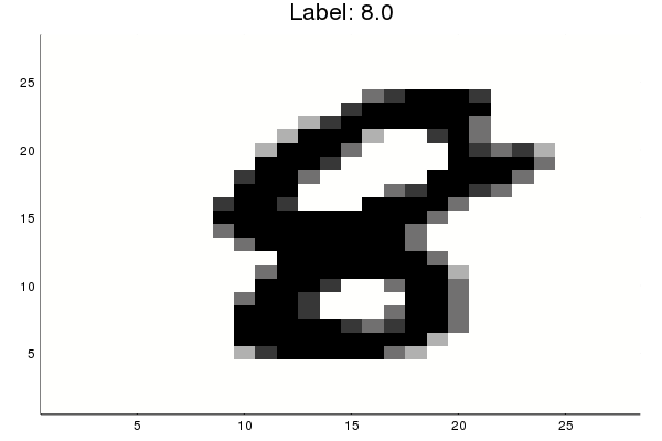
Now, let’s parse out the labels and features and look at a few examples. Show a random example and its corresponding label:
rand_number=rand(1:60000)
rand_example_features = trainfeatures(rand_number)
rand_example_label=trainlabel(rand_number)
#img=colorview(Gray,1 .-reshape(rand_example_features, (28, 28)))
#println("Label: ",rand_example_label)
#img
p1=heatmap(reverse(1 .-reshape(rand_example_features, (28, 28)),dims=1), legend=:none, c=:gray, title="Label: $rand_example_label")
The following functions normalize the features and convert the targets to a one-hot encoding. For example, if the variable contains ‘1’ in column 5, then a human rater interpreted the handwritten character as the digit ‘6’.
function preprocess_features(data_range)
    examples = zeros(Float32, length(data_range), 784)
    for i in 1:length(data_range)
        examples[i, :] = testfeatures(i)./255.0
    end
    return examples
end


function preprocess_targets(data_range)
    targets = zeros(Float32, length(data_range), 10)
    for i in 1:length(data_range)
        label = testlabel(i)
        targets[i, Int(label)+1] = 1.0
    end
    return targets
end
Let’s devide the first 10000 datasets into training and validation examples.
training_examples = preprocess_features(1:7500)
training_targets = preprocess_targets(1:7500)

validation_examples=preprocess_features(7501:10000)
validation_targets=preprocess_targets(7501:10000);
The following function converts the predicted labels (in one-hot encoding) back to a numerical label from 0 to 9.
function to1col(targets)
    reduced_targets=zeros(size(targets,1),1)
    for i=1:size(targets,1)
        reduced_targets[i]=sum( collect(0:size(targets,2)-1).*targets[i,:])
    end
    return reduced_targets
end
Task 1: Build a Linear Model for MNIST
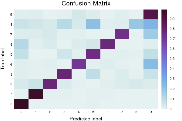
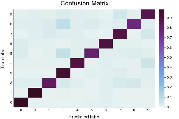
First, let’s create a baseline model to compare against. You’ll notice that in addition to reporting accuracy, and plotting Log Loss over time, we also display a confusion matrix. The confusion matrix shows which classes were misclassified as other classes. Which digits get confused for each other? Also note that we track the model’s error using the log_loss function.
function train_linear_classification_model(
    learning_rate,
    steps,
    batch_size,
    training_examples,
    training_targets,
    validation_examples,
    validation_targets)
  """Trains a linear classification model for the MNIST digits dataset.

  In addition to training, this function also prints training progress information,
  a plot of the training and validation loss over time, and a confusion
  matrix.

  Args:
    learning_rate: An `int`, the learning rate to use.
    steps: A non-zero `int`, the total number of training steps. A training step
      consists of a forward and backward pass using a single batch.
    batch_size: A non-zero `int`, the batch size.
    training_examples: An `Array` containing the training features.
    training_targets: An `Array` containing the training labels.
    validation_examples: An `Array` containing the validation features.
    validation_targets: An `Array` containing the validation labels.

  Returns:
    p1: Plot of loss metrics
    p2: Plot of confusion matrix
  """

  periods = 10

  steps_per_period = steps / periods

  # Create feature columns
  feature_columns = placeholder(Float32)
  target_columns = placeholder(Float32)

  # Create network
  W = Variable(zeros(Float32, 784, 10))
  b = Variable(zeros(Float32, 10))

  y = nn.softmax(feature_columns*W + b)
  cross_entropy = reduce_mean(-reduce_sum(target_columns .* log(y), axis=[2]))

  # Gradient decent with gradient clipping
  my_optimizer=(train.AdamOptimizer(learning_rate))
  gvs = train.compute_gradients(my_optimizer, cross_entropy)
  capped_gvs = [(clip_by_norm(grad, 5.), var) for (grad, var) in gvs]
  my_optimizer = train.apply_gradients(my_optimizer,capped_gvs)

  run(sess, global_variables_initializer())


  # Train the model, but do so inside a loop so that we can periodically assess
  # loss metrics.
  println("Training model...")
  println("LogLoss error (on validation data):")
  training_errors = []
  validation_errors = []
  for period in 1:periods
    for i=1:steps_per_period

    # Train the model, starting from the prior state.
    features_batches, targets_batches = next_batch(loader, batch_size)
    run(sess, my_optimizer, Dict(feature_columns=>features_batches, target_columns=>targets_batches))
    end

    # Take a break and compute probabilities.
    training_predictions = run(sess, y, Dict(feature_columns=> training_examples, target_columns=>training_targets))
    validation_predictions = run(sess, y, Dict(feature_columns=> validation_examples, target_columns=>validation_targets))

    # Compute training and validation errors.
    training_log_loss = sklm.log_loss(training_targets, training_predictions)
    validation_log_loss = sklm.log_loss(validation_targets, validation_predictions)
    # Occasionally print the current loss.
    println("  period ", period, ": ",validation_log_loss)
    # Add the loss metrics from this period to our list.
    push!(training_errors, training_log_loss)
    push!(validation_errors, validation_log_loss)
  end


  println("Model training finished.")

  # Calculate final predictions (not probabilities, as above).
  final_probabilities = run(sess, y, Dict(feature_columns=> validation_examples, target_columns=>validation_targets))

  final_predictions=0.0.*copy(final_probabilities)
  for i=1:size(final_predictions,1)
        final_predictions[i,argmax(final_probabilities[i,:])]=1.0
  end

  accuracy = sklm.accuracy_score(validation_targets, final_predictions)
  println("Final accuracy (on validation data): ", accuracy)

  # Output a graph of loss metrics over periods.
  p1=plot(training_errors, label="training", title="LogLoss vs. Periods", ylabel="LogLoss", xlabel="Periods")
  p1=plot!(validation_errors, label="validation")

  # Output a plot of the confusion matrix.
  cm = sklm.confusion_matrix(to1col(validation_targets), to1col(final_predictions))
  # Normalize the confusion matrix by row (i.e by the number of samples
  # in each class).
  cm_normalized=convert.(Float32,copy(cm))
  for i=1:size(cm,1)
     cm_normalized[i,:]=cm[i,:]./sum(cm[i,:])
  end
  p2 = heatmap(cm_normalized, c=:dense, title="Confusion Matrix", ylabel="True label", xlabel= "Predicted label", xticks=(1:10, 0:9), yticks=(1:10, 0:9))

  return p1, p2
end
Spend 5 minutes seeing how well you can do on accuracy with a linear model of this form. For this exercise, limit yourself to experimenting with the hyperparameters for batch size, learning rate and steps.
p1, p2 = train_linear_classification_model(
    0.02,#learning rate
    100, #steps
    10, #batch_size
    training_examples,
    training_targets,
    validation_examples,
    validation_targets)
Training model...
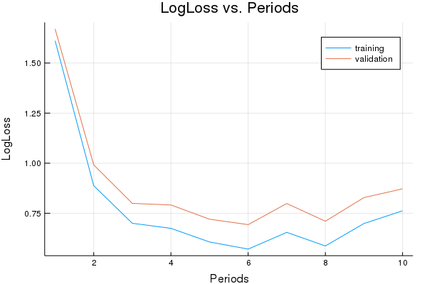
LogLoss error (on validation data):
period 1: 1.670167055553384
period 2: 0.9914946833185925
period 3: 0.7994224493201562
period 4: 0.7914848605656032
period 5: 0.7204582379937473
period 6: 0.6933409093906348
period 7: 0.7987726760530565
period 8: 0.710353285742308
period 9: 0.8285208267964786
period 10: 0.8721083970924985
Model training finished.
Final accuracy (on validation data): 0.762
plot(p1)
plot(p2)
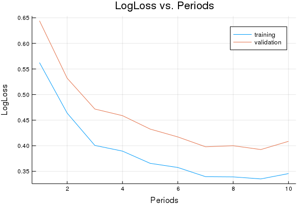
Here is a set of parameters that should attain roughly 0.9 accuracy.
sess=Session(Graph())
p1, p2 = train_linear_classification_model(
    0.003,#learning rate
    1000, #steps
    30, #batch_size
    training_examples,
    training_targets,
    validation_examples,
    validation_targets)
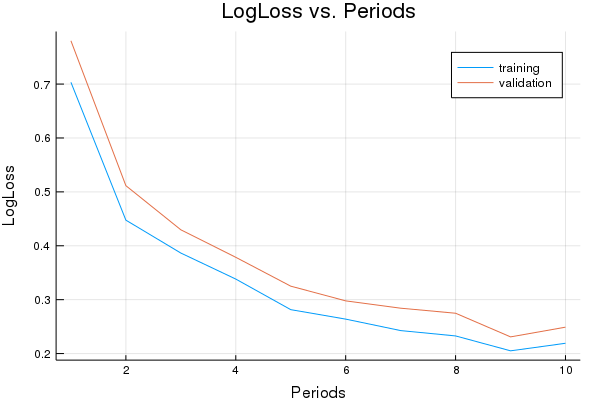
Training model...
LogLoss error (on validation data):
  period 1: 0.6441064495787024
  period 2: 0.5319821337244007
  period 3: 0.47174609823175706
  period 4: 0.4587823813826748
  period 5: 0.43256694717421595
  period 6: 0.417219959999696
  period 7: 0.39798823667723443
  period 8: 0.4000670316113661
  period 9: 0.39256970001211594
  period 10: 0.4086718587693938
Model training finished.
Final accuracy (on validation data): 0.8908
plot(p1)
plot(p2)
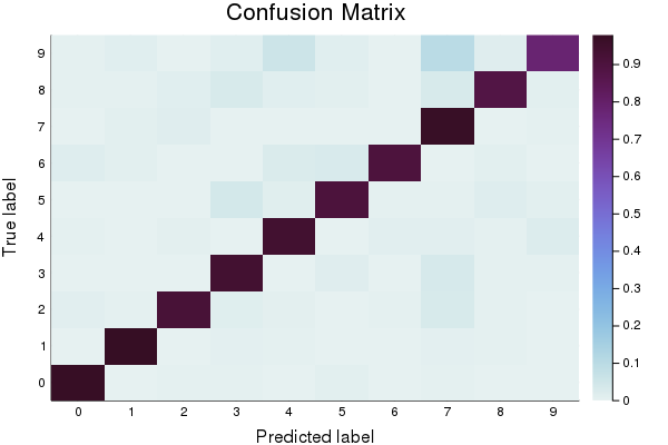
Task 2: Replace the Linear Classifier with a Neural Network
Replace the LinearClassifier above with a Neural Network and find a parameter combination that gives 0.95 or better accuracy.
You may wish to experiment with additional regularization methods, such as dropout.
The code below is almost identical to the original LinearClassifer training code, with the exception of the NN-specific configuration, such as the hyperparameter for hidden units.
function train_nn_classification_model(learning_rate,
                     steps,
                     batch_size,
                     hidden_units,
                     keep_probability,
                     training_examples,
                     training_targets,
                     validation_examples,
                     validation_targets)
  """Trains a NN classification model for the MNIST digits dataset.

  In addition to training, this function also prints training progress information,
  a plot of the training and validation loss over time, and a confusion
  matrix.

  Args:
    learning_rate: An `int`, the learning rate to use.
    steps: A non-zero `int`, the total number of training steps. A training step
      consists of a forward and backward pass using a single batch.
    batch_size: A non-zero `int`, the batch size.
    hidden_units: A vector describing the layout of the neural network.
    keep_probability: A `float`, the probability of keeping a node active during one training step.
    training_examples: An `Array` containing the training features.
    training_targets: An `Array` containing the training labels.
    validation_examples: An `Array` containing the validation features.
    validation_targets: An `Array` containing the validation labels.

  Returns:
    p1: Plot of loss metrics
    p2: Plot of confusion matrix
    y: Prediction layer of the NN.
    feature_columns: Feature column tensor of the NN.
    target_columns: Target column tensor of the NN.
    weight_export: Weights of the first layer of the NN.
  """

  periods = 10
  steps_per_period = steps / periods

  # Create feature columns.
  feature_columns = placeholder(Float32, shape=[-1, size(training_examples,2)])
  target_columns = placeholder(Float32, shape=[-1, size(training_targets,2)])

  # Network parameters
  push!(hidden_units,size(training_targets,2)) #create an output node that fits to the size of the targets
  activation_functions = Vector{Function}(undef, size(hidden_units,1))
  activation_functions[1:end-1] .= z->nn.dropout(nn.relu(z), keep_probability)
  activation_functions[end] = nn.softmax #Last function should be idenity as we need the logits

  # create network
  flag=0
  weight_export=Variable([1])
  Zs = [feature_columns]
  for (ii,(hlsize, actfun)) in enumerate(zip(hidden_units, activation_functions))
        Wii = get_variable("W_$ii"*randstring(4), [get_shape(Zs[end], 2), hlsize], Float32)
        bii = get_variable("b_$ii"*randstring(4), [hlsize], Float32)
        Zii = actfun(Zs[end]*Wii + bii)
        push!(Zs, Zii)

        if(flag==0)
            weight_export=Wii
            flag=1
        end
  end

  y=Zs[end]
  cross_entropy = reduce_mean(-reduce_sum(target_columns .* log(y), axis=[2]))

  # Standard Adam Optimizer
  my_optimizer=train.minimize(train.AdamOptimizer(learning_rate), cross_entropy)

  run(sess, global_variables_initializer())

  # Train the model, but do so inside a loop so that we can periodically assess
  # loss metrics.
  println("Training model...")
  println("LogLoss error (on validation data):")
  training_errors = []
  validation_errors = []
  for period in 1:periods
    for i=1:steps_per_period

    # Train the model, starting from the prior state.
    features_batches, targets_batches = next_batch(loader, batch_size)
    run(sess, my_optimizer, Dict(feature_columns=>features_batches, target_columns=>targets_batches))
    end

    # Take a break and compute probabilities.
    training_predictions = run(sess, y, Dict(feature_columns=> training_examples, target_columns=>training_targets))
    validation_predictions = run(sess, y, Dict(feature_columns=> validation_examples, target_columns=>validation_targets))

    # Compute training and validation errors.
    training_log_loss = sklm.log_loss(training_targets, training_predictions)
    validation_log_loss = sklm.log_loss(validation_targets, validation_predictions)
    # Occasionally print the current loss.
    println("  period ", period, ": ",validation_log_loss)
        # Add the loss metrics from this period to our list.
    push!(training_errors, training_log_loss)
    push!(validation_errors, validation_log_loss)
  end


  println("Model training finished.")

  # Calculate final predictions (not probabilities, as above).
  final_probabilities = run(sess, y, Dict(feature_columns=> validation_examples, target_columns=>validation_targets))

  final_predictions=0.0.*copy(final_probabilities)
  for i=1:size(final_predictions,1)
        final_predictions[i,argmax(final_probabilities[i,:])]=1.0
  end

  accuracy = sklm.accuracy_score(validation_targets, final_predictions)
  println("Final accuracy (on validation data): ", accuracy)

  # Output a graph of loss metrics over periods.
  p1=plot(training_errors, label="training", title="LogLoss vs. Periods", ylabel="LogLoss", xlabel="Periods")
  p1=plot!(validation_errors, label="validation")

  # Output a plot of the confusion matrix.
  cm = sklm.confusion_matrix(to1col(validation_targets), to1col(final_predictions))
  # Normalize the confusion matrix by row (i.e by the number of samples
  # in each class).
  cm_normalized=convert.(Float32,copy(cm))
  for i=1:size(cm,1)
     cm_normalized[i,:]=cm[i,:]./sum(cm[i,:])
  end

  p2 = heatmap(cm_normalized, c=:dense, title="Confusion Matrix", ylabel="True label", xlabel= "Predicted label", xticks=(1:10, 0:9), yticks=(1:10, 0:9))

  return p1, p2, y, feature_columns, target_columns, weight_export
end
sess=Session(Graph())
p1, p2, y, feature_columns, target_columns, weight_export = train_nn_classification_model(
    # TWEAK THESE VALUES TO SEE HOW MUCH YOU CAN IMPROVE THE RMSE
    0.003, #learning rate
    1000, #steps
    30, #batch_size
    [100, 100], #hidden_units
    1.0, # keep probability
    training_examples,
    training_targets,
    validation_examples,
    validation_targets)
Training model...
LogLoss error (on validation data):
  period 1: 0.7802972545112948
  period 2: 0.5114779946084309
  period 3: 0.42961612501494345
  period 4: 0.3785767363702402
  period 5: 0.3250470566823443
  period 6: 0.29775486131185236
  period 7: 0.28417328875554176
  period 8: 0.2748126428520406
  period 9: 0.23094550441845882
  period 10: 0.24898208121117577
Model training finished.
Final accuracy (on validation data): 0.9232
plot(p1)
plot(p2)
Next, we verify the accuracy on a test set.
test_examples = preprocess_features(10001:13000)
test_targets = preprocess_targets(10001:13000);
test_probabilities = run(sess, y, Dict(feature_columns=> test_examples, target_columns=>test_targets))

test_predictions=0.0.*copy(test_probabilities)
for i=1:size(test_predictions,1)
    test_predictions[i,argmax(test_probabilities[i,:])]=1.0
end

accuracy = sklm.accuracy_score(test_targets, test_predictions)
println("Accuracy on test data: ", accuracy)
Accuracy on test data: 0.9246666666666666
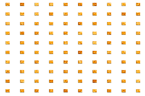
Task 3: Visualize the weights of the first hidden layer.
Let’s take a few minutes to dig into our neural network and see what it has learned by accessing the weights_export attribute of our model.
The input layer of our model has 784 weights corresponding to the 28×28 pixel input images. The first hidden layer will have 784×N weights where N is the number of nodes in that layer. We can turn those weights back into 28×28 images by reshaping each of the N 1×784 arrays of weights into N arrays of size 28×28.
Run the following cell to plot the weights. We construct a function that allows us to use a string as a variable name. This allows us to automatically name all plots. We then put together a string to display everything when evaluated.
function string_as_varname_function(s::AbstractString, v::Any)
   s = Symbol(s)
   @eval (($s) = ($v))
end

weights0 = run(sess, weight_export)

num_nodes=size(weights0,2)
num_row=convert(Int,ceil(num_nodes/10))
for i=1:num_nodes
    str_name=string("Heat",i)
    string_as_varname_function(str_name,   heatmap(reshape(weights0[:,i], (28,28)), c=:heat, legend=false, yticks=[], xticks=[] ) )
end

out_string="plot(Heat1"
for i=2:num_nodes-1
    out_string=string(out_string, ", Heat", i)
end
    out_string=string(out_string, ", Heat", num_nodes, ", layout=(num_row, 10), legend=false )")

eval(Meta.parse(out_string))
Use the following line to have a closer look at individual plots.
plot(Heat98)
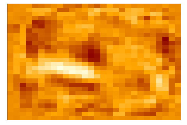
The first hidden layer of the neural network should be modeling some pretty low level features, so visualizing the weights will probably just show some fuzzy blobs or possibly a few parts of digits. You may also see some neurons that are essentially noise – these are either unconverged or they are being ignored by higher layers.
It can be interesting to stop training at different numbers of iterations and see the effect.
Train the classifier for 10, 100 and respectively 1000 steps. Then run this visualization again.
What differences do you see visually for the different levels of convergence?