This is the last exercise that uses the California housing dataset. We investigate several possibilities of optimizing neural nets:
- Different loss minimization algorithms
- Linear scaling of features
- Logarithmic scaling of features
- Clipping of features
- Z-score normalization
- Thresholding of data
The Jupyter notebook can be downloaded here.
This notebook is based on the file Improving Neural Net Performance programming exercise, which is part of Google’s Machine Learning Crash Course.
# Licensed under the Apache License, Version 2.0 (the "License");
# you may not use this file except in compliance with the License.
# You may obtain a copy of the License at
#
# https://www.apache.org/licenses/LICENSE-2.0
#
# Unless required by applicable law or agreed to in writing, software
# distributed under the License is distributed on an "AS IS" BASIS,
# WITHOUT WARRANTIES OR CONDITIONS OF ANY KIND, either express or implied.
# See the License for the specific language governing permissions and
# limitations under the License.
Improving Neural Net Performance
Learning Objective: Improve the performance of a neural network by normalizing features and applying various optimization algorithms
NOTE: The optimization methods described in this exercise are not specific to neural networks; they are effective means to improve most types of models.
Setup
First, we’ll load the data.
using Plots
using StatsPlots
using Distributions
gr(fmt=:png)
using DataFrames
using TensorFlow
import CSV
import StatsBase
using PyCall
using Random
using Statistics

sess=Session(Graph())
california_housing_dataframe = CSV.read("california_housing_train.csv", delim=",");
california_housing_dataframe = california_housing_dataframe[shuffle(1:size(california_housing_dataframe, 1)),:];
function preprocess_features(california_housing_dataframe)
  """Prepares input features from California housing data set.

  Args:
    california_housing_dataframe: A DataFrame expected to contain data
      from the California housing data set.
  Returns:
    A DataFrame that contains the features to be used for the model, including
    synthetic features.
  """
  selected_features = california_housing_dataframe[
    [:latitude,
     :longitude,
     :housing_median_age,
     :total_rooms,
     :total_bedrooms,
     :population,
     :households,
     :median_income]]
  processed_features = selected_features
  # Create a synthetic feature.
  processed_features[:rooms_per_person] = (
    california_housing_dataframe[:total_rooms] ./
    california_housing_dataframe[:population])
  return processed_features
end

function preprocess_targets(california_housing_dataframe)
  """Prepares target features (i.e., labels) from California housing data set.

  Args:
    california_housing_dataframe: A DataFrame expected to contain data
      from the California housing data set.
  Returns:
    A DataFrame that contains the target feature.
  """
  output_targets = DataFrame()
  # Scale the target to be in units of thousands of dollars.
  output_targets[:median_house_value] = (
    california_housing_dataframe[:median_house_value] ./ 1000.0)
  return output_targets
end
# Choose the first 12000 (out of 17000) examples for training.
training_examples = preprocess_features(first(california_housing_dataframe,12000))
training_targets = preprocess_targets(first(california_housing_dataframe,12000))

# Choose the last 5000 (out of 17000) examples for validation.
validation_examples = preprocess_features(last(california_housing_dataframe,5000))
validation_targets = preprocess_targets(last(california_housing_dataframe,5000))

# Double-check that we've done the right thing.
println("Training examples summary:")
describe(training_examples)
println("Validation examples summary:")
describe(validation_examples)

println("Training targets summary:")
describe(training_targets)
println("Validation targets summary:")
describe(validation_targets)
Train the Neural Network
Next, we’ll set up the neural network similar to the previous exercise.
function construct_columns(input_features)
  """Construct the TensorFlow Feature Columns.

  Args:
    input_features: DataFrame of the numerical input features to use.
  Returns:
    A set of feature columns
  """
  out=convert(Matrix, input_features[:,:])
  return convert(Matrix{Float64},out)
end
function create_batches(features, targets, steps, batch_size=5, num_epochs=0)
  """Create batches.

  Args:
    features: Input features.
    targets: Target column.
    steps: Number of steps.
    batch_size: Batch size.
    num_epochs: Number of epochs, 0 will let TF automatically calculate the correct number
  Returns:
    An extended set of feature and target columns from which batches can be extracted.
  """

    if(num_epochs==0)
        num_epochs=ceil(batch_size*steps/size(features,1))
    end

    names_features=names(features);
    names_targets=names(targets);

    features_batches=copy(features)
    target_batches=copy(targets)


    for i=1:num_epochs

        select=shuffle(1:size(features,1))

        if i==1
            features_batches=(features[select,:])
            target_batches=(targets[select,:])
        else

            append!(features_batches, features[select,:])
            append!(target_batches, targets[select,:])
        end
    end

    return features_batches, target_batches
end


function next_batch(features_batches, targets_batches, batch_size, iter)
  """Next batch.

  Args:
    features_batches: Features batches from create_batches.
    targets_batches: Target batches from create_batches.
    batch_size: Batch size.
    iter: Number of the current iteration
  Returns:
    A batch of features and targets.
  """
    select=mod((iter-1)*batch_size+1, size(features_batches,1)):mod(iter*batch_size, size(features_batches,1));

    ds=features_batches[select,:];
    target=targets_batches[select,:];

    return ds, target
end
function my_input_fn(features_batches, targets_batches, iter, batch_size=5, shuffle_flag=1)
    """Prepares a batch of features and labels for model training.

    Args:
      features_batches: Features batches from create_batches.
      targets_batches: Target batches from create_batches.
      iter: Number of the current iteration
      batch_size: Batch size.
      shuffle_flag: Determines wether data is shuffled before being returned
    Returns:
      Tuple of (features, labels) for next data batch
    """

    # Construct a dataset, and configure batching/repeating.
    ds, target = next_batch(features_batches, targets_batches, batch_size, iter)

    # Shuffle the data, if specified.
    if shuffle_flag==1
      select=shuffle(1:size(ds, 1));
        ds = ds[select,:]
        target = target[select, :]
    end

    # Return the next batch of data.
    return ds, target
end
Now we can set up the neural network itself.
function train_nn_regression_model(my_optimizer,
                     steps,
                     batch_size,
                     hidden_units,
                     keep_probability,
                     training_examples,
                     training_targets,
                     validation_examples,
                     validation_targets)
  """Trains a neural network model of one feature.

  Args:
    my_optimizer: Optimizer function for the training step
    learning_rate: A `float`, the learning rate.
    steps: A non-zero `int`, the total number of training steps. A training step
      consists of a forward and backward pass using a single batch.
    batch_size: A non-zero `int`, the batch size.
    hidden_units: A vector describing the layout of the neural network
    keep_probability: A `float`, the probability of keeping a node active during one training step.
  Returns:
    p1: Plot of RMSE for the different periods
    training_rmse: Training RMSE values for the different periods
    validation_rmse: Validation RMSE values for the different periods

  """

  periods = 10
  steps_per_period = steps / periods

  # Create feature columns.
  feature_columns = placeholder(Float32, shape=[-1, size(construct_columns(training_examples),2)])
  target_columns = placeholder(Float32, shape=[-1, size(construct_columns(training_targets),2)])

  # Network parameters
  push!(hidden_units,size(training_targets,2)) #create an output node that fits to the size of the targets
  activation_functions = Vector{Function}(undef, size(hidden_units,1))
  activation_functions[1:end-1] .= z->nn.dropout(nn.relu(z), keep_probability)
  activation_functions[end] = identity #Last function should be idenity as we need the logits

  # create network - professional template
  Zs = [feature_columns]
  for (ii,(hlsize, actfun)) in enumerate(zip(hidden_units, activation_functions))
        Wii = get_variable("W_$ii"*randstring(4), [get_shape(Zs[end], 2), hlsize], Float32)
        bii = get_variable("b_$ii"*randstring(4), [hlsize], Float32)
        Zii = actfun(Zs[end]*Wii + bii)
        push!(Zs, Zii)
  end

  y=Zs[end]
  loss=reduce_sum((target_columns - y).^2)

  features_batches, targets_batches = create_batches(training_examples, training_targets, steps, batch_size)

  # Optimizer setup with gradient clipping
  gvs = train.compute_gradients(my_optimizer, loss)
  capped_gvs = [(clip_by_norm(grad, 5.), var) for (grad, var) in gvs]
  my_optimizer = train.apply_gradients(my_optimizer,capped_gvs)

  run(sess, global_variables_initializer())

  # Train the model, but do so inside a loop so that we can periodically assess
  # loss metrics.
  println("Training model...")
  println("RMSE (on training data):")
  training_rmse = []
  validation_rmse=[]

  for period in 1:periods
    # Train the model, starting from the prior state.
   for i=1:steps_per_period
    features, labels = my_input_fn(features_batches, targets_batches, convert(Int,(period-1)*steps_per_period+i), batch_size)
    run(sess, my_optimizer, Dict(feature_columns=>construct_columns(features), target_columns=>construct_columns(labels)))
   end
    # Take a break and compute predictions.
    training_predictions = run(sess, y, Dict(feature_columns=> construct_columns(training_examples)));
    validation_predictions = run(sess, y, Dict(feature_columns=> construct_columns(validation_examples)));

    # Compute loss.
     training_mean_squared_error = mean((training_predictions- construct_columns(training_targets)).^2)
     training_root_mean_squared_error = sqrt(training_mean_squared_error)
     validation_mean_squared_error = mean((validation_predictions- construct_columns(validation_targets)).^2)
     validation_root_mean_squared_error = sqrt(validation_mean_squared_error)
    # Occasionally print the current loss.
    println("  period ", period, ": ", training_root_mean_squared_error)
    # Add the loss metrics from this period to our list.
    push!(training_rmse, training_root_mean_squared_error)
    push!(validation_rmse, validation_root_mean_squared_error)
 end

  println("Model training finished.")

  # Output a graph of loss metrics over periods.
  p1=plot(training_rmse, label="training", title="Root Mean Squared Error vs. Periods", ylabel="RMSE", xlabel="Periods")
  p1=plot!(validation_rmse, label="validation")

  #
  println("Final RMSE (on training data): ", training_rmse[end])
  println("Final RMSE (on validation data): ", validation_rmse[end])

  return  p1, training_rmse, validation_rmse
end
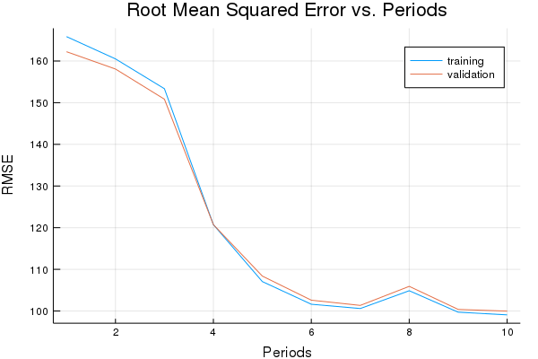
Train the model with a Gradient Descent Optimizer and a learning rate of 0.0007.
p1, training_rmse, validation_rmse = train_nn_regression_model(
    train.GradientDescentOptimizer(0.0007), #optimizer & learning rate
    5000, #steps
    70, #batch_size
    [10, 10], #hidden_units
    1.0, # keep probability
    training_examples,
    training_targets,
    validation_examples,
    validation_targets)
Training model...
RMSE (on training data):
  period 1: 165.85894301332755
  period 2: 160.50927351232303
  period 3: 153.35022496410676
  period 4: 120.72307248006544
  period 5: 107.05555881067691
  period 6: 101.61820364152953
  period 7: 100.5907723870872
  period 8: 104.86374795122849
  period 9: 99.71307532487795
  period 10: 99.07083094726671
Model training finished.
Final RMSE (on training data): 99.07083094726671
Final RMSE (on validation data): 99.97166795464649
plot(p1)
Linear Scaling
It can be a good standard practice to normalize the inputs to fall within the range -1, 1. This helps SGD not get stuck taking steps that are too large in one dimension, or too small in another. Fans of numerical optimization may note that there’s a connection to the idea of using a preconditioner here.
function linear_scale(series)
  min_val = minimum(series)
  max_val = maximum(series)
  scale = (max_val - min_val) / 2.0
  return (series .- min_val) ./ scale .- 1.0
end
Task 1: Normalize the Features Using Linear Scaling
Normalize the inputs to the scale -1, 1.
As a rule of thumb, NN’s train best when the input features are roughly on the same scale.
Sanity check your normalized data. (What would happen if you forgot to normalize one feature?)
Since normalization uses min and max, we have to ensure it’s done on the entire dataset at once.
We can do that here because all our data is in a single DataFrame. If we had multiple data sets, a good practice would be to derive the normalization parameters from the training set and apply those identically to the test set.
function normalize_linear_scale(examples_dataframe)
"""Returns a version of the input `DataFrame` that has all its features normalized linearly."""
processed_features = DataFrame()
processed_features[:latitude] = linear_scale(examples_dataframe[:latitude])
processed_features[:longitude] = linear_scale(examples_dataframe[:longitude])
processed_features[:housing_median_age] = linear_scale(examples_dataframe[:housing_median_age])
processed_features[:total_rooms] = linear_scale(examples_dataframe[:total_rooms])
processed_features[:total_bedrooms] = linear_scale(examples_dataframe[:total_bedrooms])
processed_features[:population] = linear_scale(examples_dataframe[:population])
processed_features[:households] = linear_scale(examples_dataframe[:households])
processed_features[:median_income] = linear_scale(examples_dataframe[:median_income])
processed_features[:rooms_per_person] = linear_scale(examples_dataframe[:rooms_per_person])
return processed_features
end
normalized_dataframe = normalize_linear_scale(preprocess_features(california_housing_dataframe))
normalized_training_examples = first(normalized_dataframe, 12000)
normalized_validation_examples = last(normalized_dataframe, 5000)
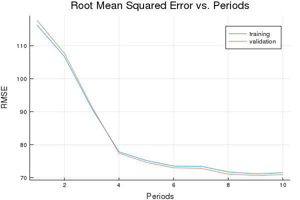
p1, graddescent_training_rmse, graddescent_validation_rmse = train_nn_regression_model(
train.GradientDescentOptimizer(0.005),
2000,
50,
[10, 10],
1.0,
normalized_training_examples,
training_targets,
normalized_validation_examples,
validation_targets)
Training model...
RMSE (on training data):
  period 1: 116.26889073500267
  period 2: 106.73640044575028
  period 3: 91.05864835286066
  period 4: 77.83690592812205
  period 5: 75.19231136749714
  period 6: 73.50497451964335
  period 7: 73.45210518001106
  period 8: 71.72622557893618
  period 9: 71.16226315317603
  period 10: 71.48133554525255
Model training finished.
Final RMSE (on training data): 71.48133554525255
Final RMSE (on validation data): 70.87402590007358
describe(normalized_dataframe)
| variable | mean | min | median | max | nunique | nmissing | eltype | |
|---|---|---|---|---|---|---|---|---|
| Symbol | Float64 | Float64 | Float64 | Float64 | Nothing | Nothing | DataType | |
| 1 | latitude | -0.344267 | -1.0 | -0.636557 | 1.0 | Float64 | ||
| 2 | longitude | -0.0462367 | -1.0 | 0.167331 | 1.0 | Float64 | ||
| 3 | housing_median_age | 0.0819354 | -1.0 | 0.0980392 | 1.0 | Float64 | ||
| 4 | total_rooms | -0.860727 | -1.0 | -0.887966 | 1.0 | Float64 | ||
| 5 | total_bedrooms | -0.832895 | -1.0 | -0.865611 | 1.0 | Float64 | ||
| 6 | population | -0.920033 | -1.0 | -0.934752 | 1.0 | Float64 | ||
| 7 | households | -0.83548 | -1.0 | -0.865812 | 1.0 | Float64 | ||
| 8 | median_income | -0.533292 | -1.0 | -0.580047 | 1.0 | Float64 | ||
| 9 | rooms_per_person | -0.928886 | -1.0 | -0.930325 | 1.0 | Float64 |
plot(p1)
Task 2: Try a Different Optimizer
Use the Momentum and Adam optimizers and compare performance.
The Momentum optimizer is one alternative. The key insight of Momentum is that a gradient descent can oscillate heavily in case the sensitivity of the model to parameter changes is very different for different model parameters. So instead of just updating the weights and biases in the direction of reducing the loss for the current step, the optimizer combines it with the direction from the previous step. You can use Momentum by specifying MomentumOptimizer instead of GradientDescentOptimizer. Note that you need to give two parameters - a learning rate and a “momentum” - with Momentum.
For non-convex optimization problems, Adam is sometimes an efficient optimizer. To use Adam, invoke the train.AdamOptimizer method. This method takes several optional hyperparameters as arguments, but our solution only specifies one of these (learning_rate). In a production setting, you should specify and tune the optional hyperparameters carefully.
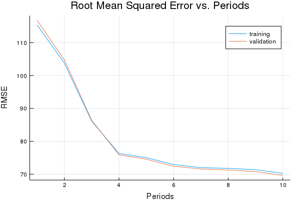
First, let’s try Momentum Optimizer.
p1, momentum_training_rmse, momentum_validation_rmse = train_nn_regression_model(
    train.MomentumOptimizer(0.005, 0.05),
    2000,
    50,
    [10, 10],
    1.0,
    normalized_training_examples,
    training_targets,
    normalized_validation_examples,
    validation_targets)
Training model...
RMSE (on training data):
  period 1: 115.40443929060348
  period 2: 103.74625375157245
  period 3: 86.13723157850293
  period 4: 76.29900844325503
  period 5: 75.01080834642302
  period 6: 72.95166497066361
  period 7: 71.98564219650198
  period 8: 71.7774064615067
  period 9: 71.36766945713532
  period 10: 70.26719355635008
Model training finished.
Final RMSE (on training data): 70.26719355635008
Final RMSE (on validation data): 69.62952431792871
plot(p1)
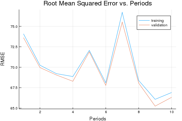
Now let’s try Adam.
p1, adam_training_rmse, adam_validation_rmse = train_nn_regression_model(
    train.AdamOptimizer(0.2),
    2000,
    50,
    [10, 10],
    1.0,
    normalized_training_examples,
    training_targets,
    normalized_validation_examples,
    validation_targets)
Training model...
RMSE (on training data):
  period 1: 74.0810426573831
  period 2: 70.2486148034969
  period 3: 69.21678023530404
  period 4: 68.86351585661589
  period 5: 72.06183656732628
  period 6: 68.09696121219436
  period 7: 76.70891547463283
  period 8: 68.38426508548561
  period 9: 66.0786086206005
  period 10: 66.91047124485922
Model training finished.
Final RMSE (on training data): 66.91047124485922
Final RMSE (on validation data): 66.3217953587637
plot(p1)
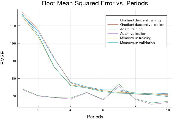
Let’s print a graph of loss metrics side by side.
p2=plot(graddescent_training_rmse, label="Gradient descent training", ylabel="RMSE", xlabel="Periods", title="Root Mean Squared Error vs. Periods")
p2=plot!(graddescent_validation_rmse, label="Gradient descent validation")
p2=plot!(adam_training_rmse, label="Adam training")
p2=plot!(adam_validation_rmse, label="Adam validation")
p2=plot!(momentum_training_rmse, label="Momentum training")
p2=plot!(momentum_validation_rmse, label="Momentum validation")
Task 3: Explore Alternate Normalization Methods
Try alternate normalizations for various features to further improve performance.
If you look closely at summary stats for your transformed data, you may notice that linear scaling some features leaves them clumped close to -1.
For example, many features have a median of -0.8 or so, rather than 0.0.
# I'd like a better solution to automate this, but all ideas for eval
# on quoted expressions failed :-()
hist1=histogram(normalized_training_examples[:latitude], bins=20,  title="latitude"  )
hist2=histogram(normalized_training_examples[:longitude], bins=20,  title="longitude"  )
hist3=histogram(normalized_training_examples[:housing_median_age], bins=20,  title="housing_median_age"  )
hist4=histogram(normalized_training_examples[:total_rooms], bins=20,  title="total_rooms"  )
hist5=histogram(normalized_training_examples[:total_bedrooms], bins=20,  title="total_bedrooms"  )
hist6=histogram(normalized_training_examples[:population], bins=20,  title="population"  )
hist7=histogram(normalized_training_examples[:households], bins=20,  title="households"  )
hist8=histogram(normalized_training_examples[:median_income], bins=20,  title="median_income"  )
hist9=histogram(normalized_training_examples[:rooms_per_person], bins=20,  title="rooms_per_person"  )

plot(hist1, hist2, hist3, hist4, hist5, hist6, hist7, hist8, hist9, layout=9, legend=false)
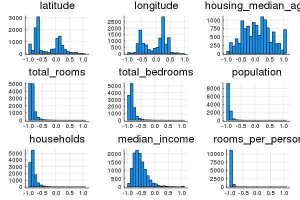
We might be able to do better by choosing additional ways to transform these features.
For example, a log scaling might help some features. Or clipping extreme values may make the remainder of the scale more informative.
function log_normalize(series)
  return log.(series.+1.0)
end

function clip(series, clip_to_min, clip_to_max)
  return min.(max.(series, clip_to_min), clip_to_max)
end

function z_score_normalize(series)
  mean_val = mean(series)
  std_dv = std(series, mean=mean_val)
  return (series .- mean) ./ std_dv
end

function binary_threshold(series, threshold)
  return map(x->(x > treshold ? 1 : 0), series)
end
The block above contains a few additional possible normalization functions.
Note that if you normalize the target, you’ll need to un-normalize the predictions for loss metrics to be comparable.
These are only a few ways in which we could think about the data. Other transformations may work even better!
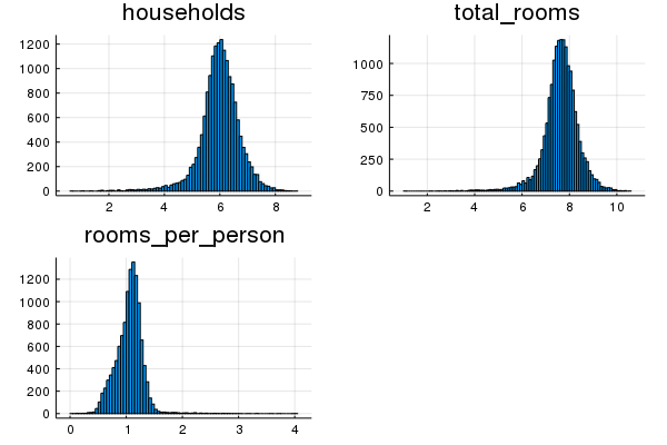
households, median_income and total_bedrooms all appear normally-distributed in a log space.
hist10=histogram(log_normalize(california_housing_dataframe[:households]), title="households")
hist11=histogram(log_normalize(california_housing_dataframe[:total_rooms]), title="total_rooms")
hist12=histogram(log_normalize(training_examples[:rooms_per_person]), title="rooms_per_person")
plot(hist10, hist11, hist12, layout=3, legend=false)
latitude, longitude and housing_median_age would probably be better off just scaled linearly, as before.
population, total_rooms and rooms_per_person have a few extreme outliers. They seem too extreme for log normalization to help. So let’s clip them instead.
function normalize_df(examples_dataframe)
  """Returns a version of the input `DataFrame` that has all its features normalized."""
  processed_features = DataFrame()

  processed_features[:households] = log_normalize(examples_dataframe[:households])
  processed_features[:median_income] = log_normalize(examples_dataframe[:median_income])
  processed_features[:total_bedrooms] = log_normalize(examples_dataframe[:total_bedrooms])

  processed_features[:latitude] = linear_scale(examples_dataframe[:latitude])
  processed_features[:longitude] = linear_scale(examples_dataframe[:longitude])
  processed_features[:housing_median_age] = linear_scale(examples_dataframe[:housing_median_age])

  processed_features[:population] = linear_scale(clip(examples_dataframe[:population], 0, 5000))
  processed_features[:rooms_per_person] = linear_scale(clip(examples_dataframe[:rooms_per_person], 0, 5))
  processed_features[:total_rooms] = linear_scale(clip(examples_dataframe[:total_rooms], 0, 10000))

  return processed_features
end

normalized_dataframe = normalize_df(preprocess_features(california_housing_dataframe))
normalized_training_examples = first(normalized_dataframe,12000)
normalized_validation_examples = last(normalized_dataframe,5000)

p1, adam_training_rmse, adam_validation_rmse = train_nn_regression_model(
    train.AdamOptimizer(0.15),
    2000,
    50,
    [10, 10],
    1.0,
    normalized_training_examples,
    training_targets,
    normalized_validation_examples,
    validation_targets)
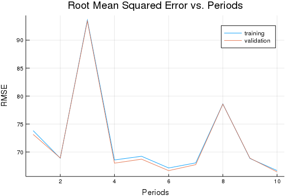
Training model...
RMSE (on training data):
  period 1: 73.81805701641049
  period 2: 68.8930841826046
  period 3: 93.6066512633055
  period 4: 68.57789741977855
  period 5: 69.23834604154376
  period 6: 67.14586221179083
  period 7: 68.05893852680245
  period 8: 78.60115010290136
  period 9: 68.84296171023885
  period 10: 66.67798003495479
Model training finished.
Final RMSE (on training data): 66.67798003495479
Final RMSE (on validation data): 66.44152260236143
plot(p1)
Optional Challenge: Use only Latitude and Longitude Features
Train a NN model that uses only latitude and longitude as features.
Real estate people are fond of saying that location is the only important feature in housing price. Let’s see if we can confirm this by training a model that uses only latitude and longitude as features.
This will only work well if our NN can learn complex nonlinearities from latitude and longitude.
NOTE: We may need a network structure that has more layers than were useful earlier in the exercise.
It’s a good idea to keep latitude and longitude normalized:
function location_location_location(examples_dataframe)
  """Returns a version of the input `DataFrame` that keeps only the latitude and longitude."""
  processed_features = DataFrame()
  processed_features[:latitude] = linear_scale(examples_dataframe[:latitude])
  processed_features[:longitude] = linear_scale(examples_dataframe[:longitude])
  return processed_features
end

lll_dataframe = location_location_location(preprocess_features(california_housing_dataframe))
lll_training_examples = first(lll_dataframe,12000)
lll_validation_examples = last(lll_dataframe,5000)

p1, lll_training_rmse, lll_validation_rmse = train_nn_regression_model(
    train.AdamOptimizer(0.15),
    500,
    100,
    [10, 10, 5, 5],
    1.0,
    lll_training_examples,
    training_targets,
    lll_validation_examples,
    validation_targets)
Training model...
RMSE (on training data):
  period 1: 111.726547580272
  period 2: 100.74697632974917
  period 3: 102.50194661623024
  period 4: 99.93336589731489
  period 5: 113.76245927957433
  period 6: 98.65038062927565
  period 7: 114.59608320942579
  period 8: 101.52184438244362
  period 9: 98.30844015794274
  period 10: 116.86833668631782
Model training finished.
Final RMSE (on training data): 116.86833668631782
Final RMSE (on validation data): 115.82879219512942
plot(p1)
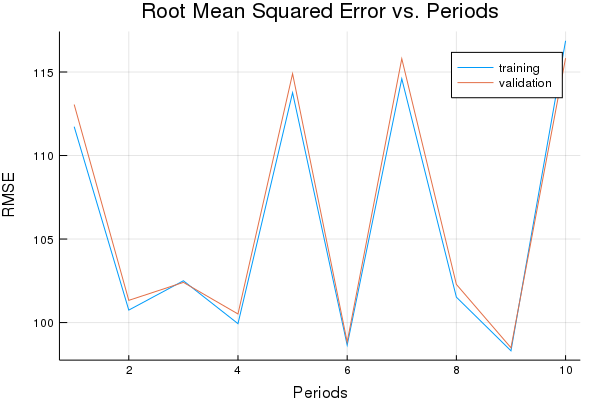
This isn’t too bad for just two features. Of course, property values can still vary significantly within short distances.