The next part of the Machine Learning Crash Course deals with Logistic Regression.
We construct the log loss function by using reduce_mean and regularizing by adding a small contant in the log function, to avoid numerical problems. The quality of the model is assessed by using some functions provided by the Python module scikit-learn. One can use
using Conda
Conda.add("scikit-learn")
to install the package. After that, it can be imported using PyCall:
using PyCall
@pyimport sklearn.metrics as sklm
The Jupyter notebook can be downloaded here.
This notebook is based on the file Logistic Regression programming exercise, which is part of Google’s Machine Learning Crash Course.
# Licensed under the Apache License, Version 2.0 (the "License");
# you may not use this file except in compliance with the License.
# You may obtain a copy of the License at
#
# https://www.apache.org/licenses/LICENSE-2.0
#
# Unless required by applicable law or agreed to in writing, software
# distributed under the License is distributed on an "AS IS" BASIS,
# WITHOUT WARRANTIES OR CONDITIONS OF ANY KIND, either express or implied.
# See the License for the specific language governing permissions and
# limitations under the License.
Logistic Regression
Learning Objectives:
- Reframe the median house value predictor (from the preceding exercises) as a binary classification model
- Compare the effectiveness of logisitic regression vs linear regression for a binary classification problem
As in the prior exercises, we’re working with the California housing data set, but this time we will turn it into a binary classification problem by predicting whether a city block is a high-cost city block. We’ll also revert to the default features, for now.
Frame the Problem as Binary Classification
The target of our dataset is median_house_value which is a numeric (continuous-valued) feature. We can create a boolean label by applying a threshold to this continuous value.
Given features describing a city block, we wish to predict if it is a high-cost city block. To prepare the targets for train and eval data, we define a classification threshold of the 75%-ile for median house value (a value of approximately 265000). All house values above the threshold are labeled 1, and all others are labeled 0.
Setup
Run the cells below to load the data and prepare the input features and targets.
using Plots
using Distributions
gr(fmt=:png)
using DataFrames
using TensorFlow
import CSV
import StatsBase
using PyCall
using Random
using Statistics

sess=Session(Graph())
california_housing_dataframe = CSV.read("california_housing_train.csv", delim=",");
california_housing_dataframe = california_housing_dataframe[shuffle(1:size(california_housing_dataframe, 1)),:];
Note how the code below is slightly different from the previous exercises. Instead of using median_house_value as target, we create a new binary target, median_house_value_is_high.
function preprocess_features(california_housing_dataframe)
  """Prepares input features from California housing data set.

  Args:
    california_housing_dataframe: A DataFrame expected to contain data
      from the California housing data set.
  Returns:
    A DataFrame that contains the features to be used for the model, including
    synthetic features.
  """
  selected_features = california_housing_dataframe[
    [:latitude,
     :longitude,
     :housing_median_age,
     :total_rooms,
     :total_bedrooms,
     :population,
     :households,
     :median_income]]
  processed_features = selected_features
  # Create a synthetic feature.
  processed_features[:rooms_per_person] = (
    california_housing_dataframe[:total_rooms] ./
    california_housing_dataframe[:population])
  return processed_features
end


function preprocess_targets(california_housing_dataframe)
  """Prepares target features (i.e., labels) from California housing data set.

  Args:
    california_housing_dataframe: A DataFrame expected to contain data
      from the California housing data set.
  Returns:
    A DataFrame that contains the target feature.
  """
  output_targets = DataFrame()
  # Scale the target to be in units of thousands of dollars.
  output_targets[:median_house_value_is_high] = convert.(Float64,
    california_housing_dataframe[:median_house_value] .> 265000)
  return output_targets
end
# Choose the first 12000 (out of 17000) examples for training.
training_examples = preprocess_features(first(california_housing_dataframe,12000))
training_targets = preprocess_targets(first(california_housing_dataframe,12000))

# Choose the last 5000 (out of 17000) examples for validation.
validation_examples = preprocess_features(last(california_housing_dataframe,5000))
validation_targets = preprocess_targets(last(california_housing_dataframe,5000))

# Double-check that we've done the right thing.
println("Training examples summary:")
describe(training_examples)
println("Validation examples summary:")
describe(validation_examples)

println("Training targets summary:")
describe(training_targets)
println("Validation targets summary:")
describe(validation_targets)
How Would Linear Regression Fare?
To see why logistic regression is effective, let us first train a naive model that uses linear regression. This model will use labels with values in the set {0, 1} and will try to predict a continuous value that is as close as possible to 0 or 1. Furthermore, we wish to interpret the output as a probability, so it would be ideal if the output will be within the range (0, 1). We would then apply a threshold of 0.5 to determine the label.
Run the cells below to train the linear regression model.
function construct_feature_columns(input_features)
  """Construct the TensorFlow Feature Columns.

  Args:
    input_features: The names of the numerical input features to use.
  Returns:
    A set of feature columns
  """
  out=convert(Matrix, input_features[:,:])
  return convert(Matrix{Float64},out)
end
function create_batches(features, targets, steps, batch_size=5, num_epochs=0)
  """Create batches.

  Args:
    features: Input features.
    targets: Target column.
    steps: Number of steps.
    batch_size: Batch size.
    num_epochs: Number of epochs, 0 will let TF automatically calculate the correct number
  Returns:
    An extended set of feature and target columns from which batches can be extracted.
  """

    if(num_epochs==0)
        num_epochs=ceil(batch_size*steps/size(features,1))
    end

    names_features=names(features);
    names_targets=names(targets);

    features_batches=copy(features)
    target_batches=copy(targets)

    for i=1:num_epochs
        select=shuffle(1:size(features,1))
        if i==1
            features_batches=(features[select,:])
            target_batches=(targets[select,:])
        else
            append!(features_batches, features[select,:])
            append!(target_batches, targets[select,:])
        end
    end
    return features_batches, target_batches
end
function next_batch(features_batches, targets_batches, batch_size, iter)
  """Next batch.

  Args:
    features_batches: Features batches from create_batches.
    targets_batches: Target batches from create_batches.
    batch_size: Batch size.
    iter: Number of the current iteration
  Returns:
    An extended set of feature and target columns from which batches can be extracted.
  """
    select=mod((iter-1)*batch_size+1, size(features_batches,1)):mod(iter*batch_size, size(features_batches,1));

    ds=features_batches[select,:];
    target=targets_batches[select,:];

    return ds, target
end
function my_input_fn(features_batches, targets_batches, iter, batch_size=5, shuffle_flag=1)
    """Prepares a batch of features and labels for model training.

    Args:
      features: DataFrame of features
      targets: DataFrame of targets
      batch_size: Size of batches to be passed to the model
      shuffle: True or False. Whether to shuffle the data.
      num_epochs: Number of epochs for which data should be repeated. None = repeat indefinitely
    Returns:
      Tuple of (features, labels) for next data batch
    """
    # Construct a dataset, and configure batching/repeating.
    ds, target = next_batch(features_batches, targets_batches, batch_size, iter)

    # Shuffle the data, if specified.
    if shuffle_flag==1
      select=shuffle(1:size(ds, 1));
        ds = ds[select,:]
        target = target[select, :]
    end

    # Return the next batch of data.
    return ds, target
end
function train_linear_regressor_model(learning_rate,
steps,
batch_size,
training_examples,
training_targets,
validation_examples,
validation_targets)
"""Trains a linear regression model of one feature.
Args:
learning_rate: A `float`, the learning rate.
steps: A non-zero `int`, the total number of training steps. A training step
consists of a forward and backward pass using a single batch.
batch_size: A non-zero `int`, the batch size.
training_examples:
training_targets:
validation_examples:
validation_targets:
Returns:
weight: The weights of the model.
bias: Bias of the model.
p1: Graph containing the loss function values for the different iterations.
"""
periods = 10
steps_per_period = steps / periods
# Create feature columns.
feature_columns = placeholder(Float32)
target_columns = placeholder(Float32)
# Create a linear regressor object.
m=Variable(zeros(size(training_examples,2),1))
b=Variable(0.0)
y=(feature_columns*m) .+ b
loss=reduce_sum((target_columns - y).^2)
features_batches, targets_batches = create_batches(training_examples, training_targets, steps, batch_size)
# Use gradient descent as the optimizer for training the model.
# Advanced gradient decent with gradient clipping
my_optimizer=(train.GradientDescentOptimizer(learning_rate))
gvs = train.compute_gradients(my_optimizer, loss)
capped_gvs = [(clip_by_norm(grad, 5.), var) for (grad, var) in gvs]
my_optimizer = train.apply_gradients(my_optimizer,capped_gvs)
run(sess, global_variables_initializer())
# Train the model, but do so inside a loop so that we can periodically assess
# loss metrics.
println("Training model...")
println("RMSE (on training data):")
training_rmse = []
validation_rmse=[]
for period in 1:periods
# Train the model, starting from the prior state.
for i=1:steps_per_period
features, labels = my_input_fn(features_batches, targets_batches, convert(Int,(period-1)*steps_per_period+i), batch_size)
run(sess, my_optimizer, Dict(feature_columns=>construct_feature_columns(features), target_columns=>construct_feature_columns(labels)))
end
# Take a break and compute predictions.
training_predictions = run(sess, y, Dict(feature_columns=> construct_feature_columns(training_examples)));
validation_predictions = run(sess, y, Dict(feature_columns=> construct_feature_columns(validation_examples)));
# Compute loss.
training_mean_squared_error = mean((training_predictions- construct_feature_columns(training_targets)).^2)
training_root_mean_squared_error = sqrt(training_mean_squared_error)
validation_mean_squared_error = mean((validation_predictions- construct_feature_columns(validation_targets)).^2)
validation_root_mean_squared_error = sqrt(validation_mean_squared_error)
# Occasionally print the current loss.
println(" period ", period, ": ", training_root_mean_squared_error)
# Add the loss metrics from this period to our list.
push!(training_rmse, training_root_mean_squared_error)
push!(validation_rmse, validation_root_mean_squared_error)
end
weight = run(sess,m)
bias = run(sess,b)
println("Model training finished.")
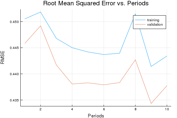
# Output a graph of loss metrics over periods.
p1=plot(training_rmse, label="training", title="Root Mean Squared Error vs. Periods", ylabel="RMSE", xlabel="Periods")
p1=plot!(validation_rmse, label="validation")
println("Final RMSE (on training data): ", training_rmse[end])
println("Final Weight (on training data): ", weight)
println("Final Bias (on training data): ", bias)
return weight, bias, p1 #, calibration_data
end
weight, bias, p1 = train_linear_regressor_model(
    0.000001, #learning rate
    200, #steps
    20, #batch_size
    training_examples,
    training_targets,
    validation_examples,
    validation_targets)
Training model...
RMSE (on training data):
  period 1: 0.45051341666072875
  period 2: 0.45182177085209174
  period 3: 0.44677893375310757
  period 4: 0.44500355042433554
  period 5: 0.4441858553929224
  period 6: 0.4436945450616647
  period 7: 0.4439450480963754
  period 8: 0.45147257346713643
  period 9: 0.4414136722731065
  period 10: 0.4434176213764645
Model training finished.
Final RMSE (on training data): 0.4434176213764645
Final Weight (on training data): [1.0837e-5; -3.77549e-5; 1.4566e-5; 0.000127498; -1.4785e-5; -9.54911e-5; 4.20284e-6; 2.93941e-6; 8.78804e-7]
Final Bias (on training data): 0.0004503312421493125
plot(p1)
Task 1: Can We Calculate LogLoss for These Predictions?
Examine the predictions and decide whether or not we can use them to calculate LogLoss.
A linear regression model uses the L2 loss, which doesn’t do a great job at penalizing misclassifications when the output is interpreted as a probability. For example, there should be a huge difference whether a negative example is classified as positive with a probability of 0.9 vs 0.9999, but L2 loss doesn’t strongly differentiate these cases.
In contrast, LogLoss penalizes these “confidence errors” much more heavily. Remember, LogLoss is defined as:
But first, we’ll need to obtain the prediction values. We could use LinearRegressor.predict to obtain these.
Given the predictions and that targets, can we calculate LogLoss?
Solution
Click below to display the solution.
validation_predictions = (construct_feature_columns(validation_examples)*weight .+ bias) .> 0.5
convert.(Float64, validation_predictions)

eps=1E-8
validation_log_loss=-mean(log.(validation_predictions.+eps).*construct_feature_columns(validation_targets) + log.(1 .-validation_predictions.+eps).*(1 .-construct_feature_columns(validation_targets)))
4.726746671464179
Task 2: Train a Logistic Regression Model and Calculate LogLoss on the Validation Set
To use logistic regression, we construct a model with a log loss function below.
function train_linear_classifier_model(learning_rate,
steps,
batch_size,
training_examples,
training_targets,
validation_examples,
validation_targets)
"""Trains a linear classifier model of one feature.
Args:
learning_rate: A `float`, the learning rate.
steps: A non-zero `int`, the total number of training steps. A training step
consists of a forward and backward pass using a single batch.
batch_size: A non-zero `int`, the batch size.
training_examples:
training_targets:
validation_examples:
validation_targets:
Returns:
weight: The weights of the model.
bias: Bias of the model.
validation_probabilities: Probabilities for the validation data.
p1: Graph containing the loss function values for the different iterations.
"""
periods = 10
steps_per_period = steps / periods
# Create feature columns.
feature_columns = placeholder(Float32)
target_columns = placeholder(Float32)
eps=1E-8
# Create a linear classifier object.
# Configure the linear regression model with our feature columns and optimizer.
m=Variable(zeros(size(training_examples,2),1).+0.0)
b=Variable(0.0)
ytemp=nn.sigmoid(feature_columns*m + b)
y= clip_by_value(ytemp, 0.0, 1.0)
loss = -reduce_mean(log(y+eps).*target_columns + log(1-y+eps).*(1-target_columns))
features_batches, targets_batches = create_batches(training_examples, training_targets, steps, batch_size)
# Adam optimizer with gradient clipping
my_optimizer=(train.AdamOptimizer(learning_rate))
gvs = train.compute_gradients(my_optimizer, loss)
capped_gvs = [(clip_by_norm(grad, 5.0), var) for (grad, var) in gvs]
my_optimizer = train.apply_gradients(my_optimizer,capped_gvs)
run(sess, global_variables_initializer()) #this needs to be run after constructing the optimizer!
# Train the model, but do so inside a loop so that we can periodically assess
# loss metrics.
println("Training model...")
println("LogLoss (on training data):")
training_log_losses = []
validation_log_losses=[]
for period in 1:periods
# Train the model, starting from the prior state.
for i=1:steps_per_period
features, labels = my_input_fn(features_batches, targets_batches, convert(Int,(period-1)*steps_per_period+i), batch_size)
run(sess, my_optimizer, Dict(feature_columns=>construct_feature_columns(features), target_columns=>construct_feature_columns(labels)))
end
# Take a break and compute predictions.
training_probabilities = run(sess, y, Dict(feature_columns=> construct_feature_columns(training_examples)));
validation_probabilities = run(sess, y, Dict(feature_columns=> construct_feature_columns(validation_examples)));
# Compute loss.
training_log_loss=run(sess,loss,Dict(feature_columns=> construct_feature_columns(training_examples), target_columns=>construct_feature_columns(training_targets)))
validation_log_loss =run(sess,loss,Dict(feature_columns=> construct_feature_columns(validation_examples), target_columns=>construct_feature_columns(validation_targets)))
# Occasionally print the current loss.
println(" period ", period, ": ", training_log_loss)
weight = run(sess,m)
bias = run(sess,b)
loss_val=run(sess,loss,Dict(feature_columns=> construct_feature_columns(training_examples), target_columns=>construct_feature_columns(training_targets)))
# Add the loss metrics from this period to our list.
push!(training_log_losses, training_log_loss)
push!(validation_log_losses, validation_log_loss)
end
weight = run(sess,m)
bias = run(sess,b)
println("Model training finished.")
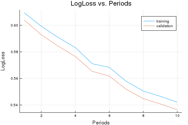
# Output a graph of loss metrics over periods.
p1=plot(training_log_losses, label="training", title="LogLoss vs. Periods", ylabel="LogLoss", xlabel="Periods")
p1=plot!(validation_log_losses, label="validation")
println("Final LogLoss (on training data): ", training_log_losses[end])
# calculate additional ouputs
validation_probabilities = run(sess, y, Dict(feature_columns=> construct_feature_columns(validation_examples)));
return weight, bias, validation_probabilities, p1 #, calibration_data
end
weight, bias, validation_probabilities,  p1 = train_linear_classifier_model(
    0.000005, #learning rate
    500, #steps
    20, #batch_size
    training_examples,
    training_targets,
    validation_examples,
    validation_targets)
Training model...
LogLoss (on training data):
  period 1: 0.6094288971718198
  period 2: 0.599245330619635
  period 3: 0.5907661769938415
  period 4: 0.5833044266780119
  period 5: 0.5710450766404077
  period 6: 0.5683473572721645
  period 7: 0.5578244955218272
  period 8: 0.5504936047681086
  period 9: 0.5465360894364992
  period 10: 0.5420948374829867
Model training finished.
Final LogLoss (on training data): 0.5420948374829867
plot(p1)
Task 3: Calculate Accuracy and plot a ROC Curve for the Validation Set
A few of the metrics useful for classification are the model accuracy, the ROC curve and the area under the ROC curve (AUC). We’ll examine these metrics.
First, we need to convert probabilities back to 0/1 labels:
# Function for converting probabilities to 0/1 decision
function castto01(probabilities)
    out=copy(probabilities)
    for i=1:length(probabilities)
        if(probabilities[i]<0.5)
            out[i]=0
        else
            out[i]=1
        end
    end
    return out
end
We use sklearn’s metric functions to calculate the ROC curve.
sklm=pyimport("sklearn.metrics")
evaluation_metrics=DataFrame()
false_positive_rate, true_positive_rate, thresholds = sklm.roc_curve(
vec(construct_feature_columns(validation_targets)), vec(validation_probabilities))
evaluation_metrics[:auc]=sklm.roc_auc_score(construct_feature_columns(validation_targets), vec(validation_probabilities))
validation_predictions=castto01(validation_probabilities);
evaluation_metrics[:accuracy]=sum(1 .-(construct_feature_columns(validation_targets)-validation_predictions))/length(validation_predictions);
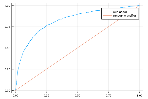
p2=plot(false_positive_rate, true_positive_rate, label="our model")
p2=plot!([0, 1], [0, 1], label="random classifier");
#evaluation_metrics = linear_classifier.evaluate(input_fn=predict_validation_input_fn)
println("AUC on the validation set: ",  evaluation_metrics[:auc])
println("Accuracy on the validation set: ", evaluation_metrics[:accuracy])
AUC on the validation set: [0.681192]
Accuracy on the validation set: [0.7672]
plot(p2)
See if you can tune the learning settings of the model trained at Task 2 to improve AUC.
Often, certain metrics improve at the detriment of others, and you’ll need to find the settings that achieve a good compromise.
Verify if all metrics improve at the same time.
One possible solution that works is to just train for longer, as long as we don’t overfit.
We can do this by increasing the number the steps, the batch size, or both.
All metrics improve at the same time, so our loss metric is a good proxy for both AUC and accuracy.
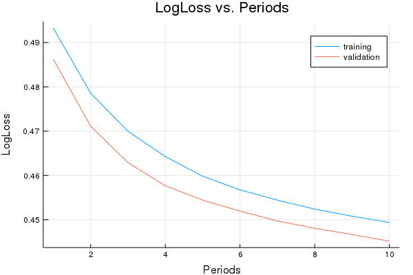
Notice how it takes many, many more iterations just to squeeze a few more units of AUC. This commonly happens. But often even this small gain is worth the costs.
# TUNE THE SETTINGS BELOW TO IMPROVE AUC
weight, bias, validation_probabilities, p1 = train_linear_classifier_model(
0.000003, #learning rate
20000, #steps
500, #batch_size
training_examples,
training_targets,
validation_examples,
validation_targets)
evaluation_metrics=DataFrame()
validation_predictions=castto01(validation_probabilities);
evaluation_metrics[:accuracy]=sum(1 .-(construct_feature_columns(validation_targets)-validation_predictions))/length(validation_predictions);
evaluation_metrics[:auc]=sklm.roc_auc_score(construct_feature_columns(validation_targets), vec(validation_probabilities))
false_positive_rate, true_positive_rate, thresholds = sklm.roc_curve(
vec(construct_feature_columns(validation_targets)), vec(validation_probabilities))
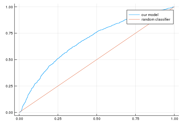
p2=plot(false_positive_rate, true_positive_rate, label="our model")
p2=plot!([0, 1], [0, 1], label="random classifier");
println("AUC on the validation set: ", evaluation_metrics[:auc])
println("Accuracy on the validation set: ", evaluation_metrics[:accuracy])
Training model...
LogLoss (on training data):
  period 1: 0.493267901770338
  period 2: 0.4785776549933992
  period 3: 0.46996659641396493
  period 4: 0.4642673725732476
  period 5: 0.45983209741733316
  period 6: 0.4567572559867093
  period 7: 0.4544268354348158
  period 8: 0.4524115786296243
  period 9: 0.45081088667431535
  period 10: 0.449398109543153
Model training finished.
Final LogLoss (on training data): 0.449398109543153
AUC on the validation set: [0.821896]
Accuracy on the validation set: [0.8642]
plot(p1)
plot(p2)