This is the final exercise of Google’s Machine Learning Crash Course. We use the ACL 2011 IMDB dataset to train a Neural Network in predicting wether a movie review is favourable or not, based on the words used in the review text.
There are two notable differences from the original exercise:
- We do not build a proper input pipeline for the data. This creates a lot of computational overhead - in principle, we need to preprocess the whole dataset before we start training the network. In practise, this if often not feasible. It would be interesting to see how such a pipeline can be implemented for TensorFlow.jl. The Julia package MLLabelUtils.jl might come handy for this task.
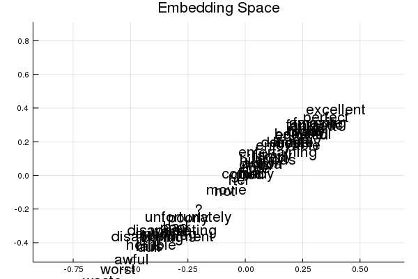
- When visualizing the embedding layer, our Neural Network builds effectively a 1D-representation of keywords to describe if a movie has a favorable review or not. In the Python version, a real 2D embedding is obtained (see the pictures). The reasons for this difference are unknown.
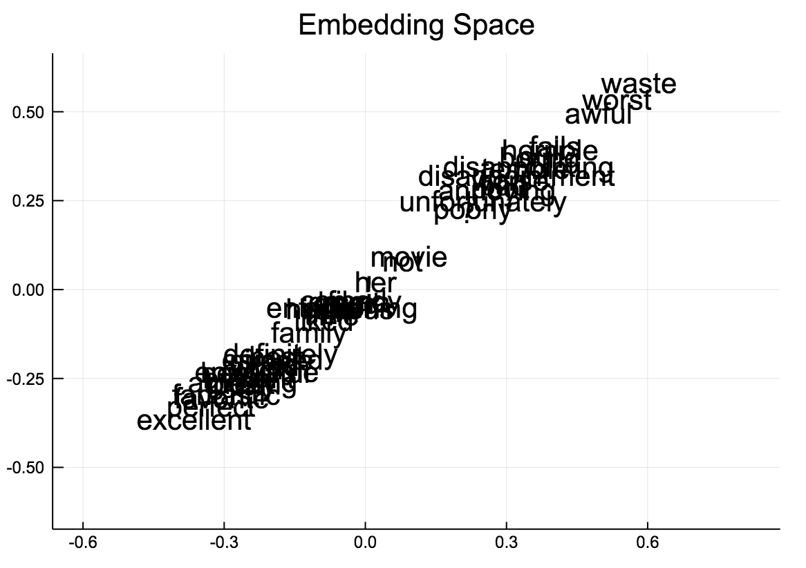 Julia embedding - effectively a 1D line
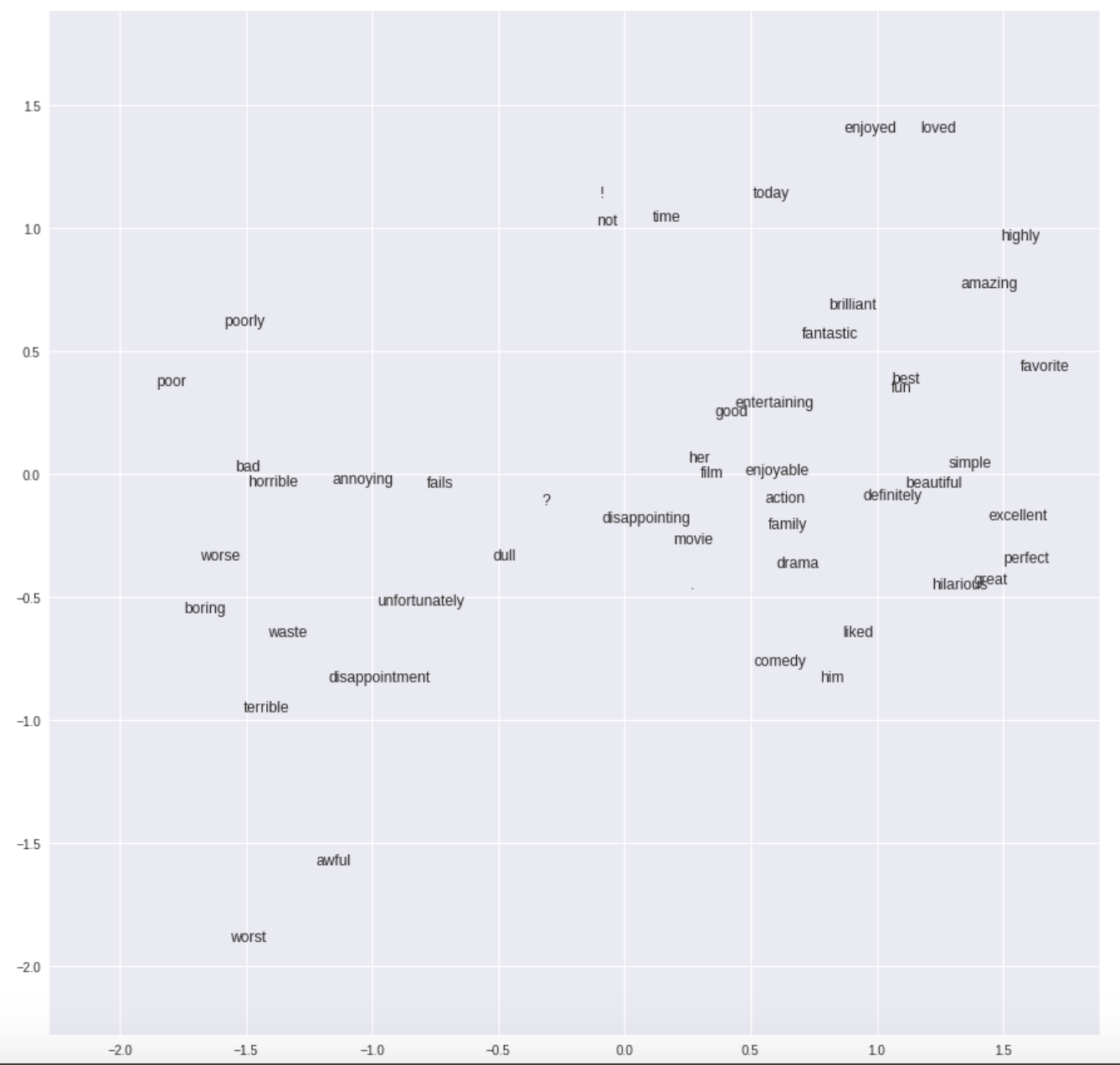 Python embedding
The Jupyter notebook can be downloaded here.
This notebook is based on the file Embeddings programming exercise, which is part of Google’s Machine Learning Crash Course.
# Licensed under the Apache License, Version 2.0 (the "License");
# you may not use this file except in compliance with the License.
# You may obtain a copy of the License at
#
# https://www.apache.org/licenses/LICENSE-2.0
#
# Unless required by applicable law or agreed to in writing, software
# distributed under the License is distributed on an "AS IS" BASIS,
# WITHOUT WARRANTIES OR CONDITIONS OF ANY KIND, either express or implied.
# See the License for the specific language governing permissions and
# limitations under the License.
Intro to Sparse Data and Embeddings
Learning Objectives:
- Convert movie-review string data to a feature vector
- Implement a sentiment-analysis linear model using a feature vector
- Implement a sentiment-analysis DNN model using an embedding that projects data into two dimensions
- Visualize the embedding to see what the model has learned about the relationships between words
In this exercise, we’ll explore sparse data and work with embeddings using text data from movie reviews (from the ACL 2011 IMDB dataset). Open and run TFrecord Extraction.ipynb Colaboratory notebook to extract the data from the original .tfrecord file as Julia variables.
Setup
Let’s import our dependencies and open the training and test data. We have exported the test and training data as hdf5 files in the previous step, so we use the HDF5-package to load the data.
using Plots
using Distributions
gr(fmt=:png)
using DataFrames
using TensorFlow
import CSV
import StatsBase
using PyCall
sklm=pyimport("sklearn.metrics")
using Images
using Colors
using Random
using Statistics
using SparseArrays
using HDF5

sess=Session()
Open the test and training raw data sets.
c = h5open("train_data.h5", "r") do file
   global train_labels=read(file, "output_labels")
   global train_features=read(file, "output_features")
end
c = h5open("test_data.h5", "r") do file
   global test_labels=read(file, "output_labels")
   global test_features=read(file, "output_features")
end
train_labels=train_labels'
test_labels=test_labels';
Have a look at one data set:
test_labels[301,:]
1-element Array{Float32,1}:
 1.0
test_features[301]
"['\"' 'don' \"'\" 't' 'change' 'your' 'husband' '\"' 'is' 'another' 'soap'\n 'opera' 'comedy' 'from' 'producer' '/' 'director' 'cecil' 'b' '.' 'de'\n 'mille' '.' 'it' 'is' 'notable' 'as' 'the' 'first' 'of' 'several' 'films'\n 'he' 'made' 'starring' 'gloria' 'swanson' '.' 'i' 'guess' 'you' 'could'\n 'also' 'call' 'it' 'a' 'sequel' 'of' 'sorts' 'to' 'his' '\"' 'old' 'wives'\n 'for' 'new' '\"' '(' '####' ')' '.' 'james' '(' 'elliot' 'dexter' ')'\n 'and' 'leila' '(' 'swanson' ')' 'porter' 'are' 'a' 'fortyish' 'couple'\n 'where' 'james' 'has' 'gone' 'to' 'seed' 'and' 'become' 'slovenly' 'and'\n 'lazy' '.' 'he' 'has' 'a' 'penchant' 'for' 'smelly' 'cigars' 'and'\n 'eating' 'raw' 'onions' '.' 'he' 'takes' 'his' 'wife' 'for' 'granted' '.'\n 'leila' 'tries' 'to' 'get' 'him' 'to' 'straighten' 'out' 'to' 'no'\n 'avail' '.' 'one' 'night' 'at' 'a' 'dinner' 'party' 'at' 'the' 'porters'\n ',' 'leila' 'meets' 'the' 'dashing' 'schyler' 'van' 'sutphen' '(' 'now'\n \"there's\" 'a' 'moniker' ')' ',' 'the' 'playboy' 'nephew' 'of' 'socialite'\n 'mrs' '.' 'huckney' '(' 'sylvia' 'ashton' ')' '.' 'she' 'invites' 'leila'\n 'to' 'her' 'home' 'for' 'the' 'weekend' 'to' 'make' 'james' '\"' 'miss'\n 'her' '\"' '.' 'once' 'there' 'schyler' 'begins' 'to' 'put' 'the' 'moves'\n 'on' 'her' ',' 'promising' 'her' 'pleasure' ',' 'wealth' 'and' 'love' ','\n 'if' 'she' 'will' 'leave' 'her' 'husband' 'and' 'go' 'with' 'him' '.'\n 'the' 'sequences' 'involving' \"leila's\" 'imagining' 'this' 'promised'\n 'new' 'life' 'are' 'lavishly' 'staged' 'and' 'forecast' 'de' \"mille's\"\n 'epic' 'costume' 'drams' 'later' 'in' 'his' 'career' '.' 'leila' ','\n 'bored' 'with' 'her' 'marriage' 'and' 'her' 'disinterested' 'husband' ','\n 'divorces' 'james' 'and' 'marries' 'the' 'playboy' '.' 'james'\n 'ultimately' 'realizes' 'that' 'he' 'has' 'lost' 'the' 'only' 'thing'\n 'that' 'mattered' 'to' 'him' 'and' 'begins' 'to' 'mend' 'his' 'ways' '.'\n 'he' 'shaves' 'off' 'his' 'mustache' ',' 'works' 'out' ',' 'shuns'\n 'onions' 'and' 'reacquires' 'some' 'manners' '.' 'meanwhile' ',' 'all'\n 'is' 'not' 'rosy' 'with' \"leila's\" 'new' 'marriage' '.' 'schyler' 'it'\n 'seems' 'likes' 'to' 'gamble' 'and' 'has' 'taken' 'up' 'with' 'the'\n 'gold' 'digging' 'nanette' '(' 'aka' 'tootsie' ',' 'or' 'some' 'such'\n 'name' ')' '(' 'julia' 'faye' ')' '.' 'schyler' 'loses' 'all' 'of' 'his'\n 'money' 'and' 'steals' \"leila's\" 'diamond' 'ring' 'to' 'cover' 'his'\n 'losses' '.' 'one' 'fateful' 'day' ',' 'leila' 'meets' 'the' '\"' 'new'\n '\"' 'james' 'and' 'is' 'taken' 'by' 'the' 'changes' 'in' 'him' '.'\n 'james' 'drives' 'her' 'home' 'and' 'becomes' 'aware' 'of' 'her'\n 'situation' 'and' '.' '.' '.' '.' '.' '.' '.' '.' '.' '.' '.' '.' '.' '.'\n '.' '.' '.' '.' '.' '.' '.' '.' '.' '.' '.' '.' '.' '.' '.' '.' '.' '.'\n '.' '.' '.' '.' '.' '.' '.' '.' '.' '.' '.' '.' '.' '.' '.' '.' '.'\n 'this' 'film' 'marked' 'the' 'beginning' 'of' 'gloria' \"swanson's\" 'rise'\n 'to' 'super' 'stardom' 'in' 'a' 'career' 'that' 'would' 'rival' 'that'\n 'of' 'mary' 'pickford' '.' 'barely' '##' 'years' 'of' 'age' ',' 'she'\n 'had' 'begun' 'her' 'career' 'in' 'mack' 'sennett' 'two' 'reel'\n 'comedies' 'as' 'a' 'teen' 'ager' '.' 'elliot' 'dexter' 'was' 'almost'\n '##' 'at' 'this' 'time' 'but' 'he' 'and' 'swanson' 'make' 'a' 'good'\n 'team' ',' 'although' \"it's\" 'hard' 'to' 'imagine' 'anyone' 'tiring' 'of'\n 'the' 'lovely' 'miss' 'swanson' 'as' 'is' 'the' 'case' 'in' 'this' 'film'\n '.' 'dexter' 'and' 'sylvia' 'ashton' 'had' 'appeared' 'in' 'the'\n 'similar' '\"' 'old' 'wives' 'for' 'new' '\"' 'where' 'the' 'wife' 'had'\n 'gone' 'to' 'seed' 'and' 'the' 'husband' 'was' 'wronged' '.' 'also' 'in'\n 'the' 'cast' 'are' 'de' 'mille' 'regulars' 'theodore' 'roberts' 'as' 'a'\n 'bishop' 'and' 'raymond' 'hatton' 'as' 'a' 'gambler' '.']"
Building a Sentiment Analysis Model
Let’s train a sentiment-analysis model on this data that predicts if a review is generally favorable (label of 1) or unfavorable (label of 0).
To do so, we’ll turn our string-value terms into feature vectors by using a vocabulary, a list of each term we expect to see in our data. For the purposes of this exercise, we’ve created a small vocabulary that focuses on a limited set of terms. Most of these terms were found to be strongly indicative of favorable or unfavorable, but some were just added because they’re interesting.
Each term in the vocabulary is mapped to a coordinate in our feature vector. To convert the string-value terms for an example into this vector format, we encode such that each coordinate gets a value of 0 if the vocabulary term does not appear in the example string, and a value of 1 if it does. Terms in an example that don’t appear in the vocabulary are thrown away.
NOTE: We could of course use a larger vocabulary, and there are special tools for creating these. In addition, instead of just dropping terms that are not in the vocabulary, we can introduce a small number of OOV (out-of-vocabulary) buckets to which you can hash the terms not in the vocabulary. We can also use a feature hashing approach that hashes each term, instead of creating an explicit vocabulary. This works well in practice, but loses interpretability, which is useful for this exercise.
Building the Input Pipeline
First, let’s configure the input pipeline to import our data into a TensorFlow model. We can use the following function to parse the training and test data and return an array of the features and the corresponding labels.
function create_batches(features, targets, steps, batch_size=5, num_epochs=0)
  """Create batches.

  Args:
    features: Input features.
    targets: Target column.
    steps: Number of steps.
    batch_size: Batch size.
    num_epochs: Number of epochs, 0 will let TF automatically calculate the correct number
  Returns:
    An extended set of feature and target columns from which batches can be extracted.
  """
    if(num_epochs==0)
        num_epochs=ceil(batch_size*steps/size(features,1))
    end

    features_batches=copy(features)
    target_batches=copy(targets)

    for i=1:num_epochs
        select=shuffle(1:size(features,1))
        if i==1
            features_batches=(features[select,:])
            target_batches=(targets[select,:])
        else
            features_batches=vcat(features_batches, features[select,:])
            target_batches=vcat(target_batches, targets[select,:])
        end
    end
    return features_batches, target_batches
end
function construct_feature_columns(input_features)
  """Construct the TensorFlow Feature Columns.

  Args:
    input_features: The numerical input features to use.
  Returns:
    A set of feature columns
  """
  out=convert(Matrix, input_features[:,:])
  return convert(Matrix{Float64},out)
end
function next_batch(features_batches, targets_batches, batch_size, iter)
  """Next batch.

  Args:
    features_batches: Features batches from create_batches.
    targets_batches: Target batches from create_batches.
    batch_size: Batch size.
    iter: Number of the current iteration
  Returns:
    A batch of features and targets.
  """
    select=mod((iter-1)*batch_size+1, size(features_batches,1)):mod(iter*batch_size, size(features_batches,1));

    ds=features_batches[select,:];
    target=targets_batches[select,:];

    return ds, target
end
function my_input_fn(features_batches, targets_batches, iter, batch_size=5, shuffle_flag=1)
    """Prepares a batch of features and labels for model training.

    Args:
      features_batches: Features batches from create_batches.
      targets_batches: Target batches from create_batches.
      iter: Number of the current iteration
      batch_size: Batch size.
      shuffle_flag: Determines wether data is shuffled before being returned
    Returns:
      Tuple of (features, labels) for next data batch
    """

    # Construct a dataset, and configure batching/repeating.
    ds, target = next_batch(features_batches, targets_batches, batch_size, iter)

    # Shuffle the data, if specified.
    if shuffle_flag==1
      select=shuffle(1:size(ds, 1));
        ds = ds[select,:]
        target = target[select, :]
    end

    # Return the next batch of data.
    return ds, target
end
Task 1: Use a Linear Model with Sparse Inputs and an Explicit Vocabulary
For our first model, we’ll build a Linear Classifier model using 50 informative terms; always start simple!
The following code constructs the feature column for our terms.
# 50 informative terms that compose our model vocabulary
informative_terms = ["bad", "great", "best", "worst", "fun", "beautiful",
                     "excellent", "poor", "boring", "awful", "terrible",
                     "definitely", "perfect", "liked", "worse", "waste",
                     "entertaining", "loved", "unfortunately", "amazing",
                     "enjoyed", "favorite", "horrible", "brilliant", "highly",
                     "simple", "annoying", "today", "hilarious", "enjoyable",
                     "dull", "fantastic", "poorly", "fails", "disappointing",
                     "disappointment", "not", "him", "her", "good", "time",
                     "?", ".", "!", "movie", "film", "action", "comedy",
                     "drama", "family"]
The following function takes the input data and vocabulary and converts the data to a one-hot encoded matrix.
# function for creating categorial colum from vocabulary list in one hot encoding
function create_data_columns(data, informative_terms)
   onehotmat=zeros(length(data), length(informative_terms))

    for i=1:length(data)
        string=data[i]
        for j=1:length(informative_terms)
            if occursin(informative_terms[j],string)
                onehotmat[i,j]=1
            end
        end
    end
    return onehotmat
end
train_feature_mat=create_data_columns(train_features, informative_terms)
test_features_mat=create_data_columns(test_features, informative_terms);
Next, we’ll construct the Linear Classifier model, train it on the training set, and evaluate it on the evaluation set. After you read through the code, run it and see how you do.
function train_linear_classifier_model(learning_rate,
steps,
batch_size,
training_examples,
training_targets,
validation_examples,
validation_targets)
"""Trains a linear classifier model.
Args:
learning_rate: A `float`, the learning rate.
steps: A non-zero `int`, the total number of training steps. A training step
consists of a forward and backward pass using a single batch.
batch_size: A non-zero `int`, the batch size.
training_examples, etc: The input data.
Returns:
weight: The weights of the linear model.
bias: The bias of the linear model.
validation_probabilities: Probabilities for the validation examples.
p1: Plot of loss function for the different periods
"""
periods = 10
steps_per_period = steps / periods
# Create feature columns.
feature_columns = placeholder(Float32)
target_columns = placeholder(Float32)
eps=1E-8
# these two variables need to be initialized as 0, otherwise method gives problems
m=Variable(zeros(size(training_examples,2),1).+0.0)
b=Variable(0.0)
ytemp=nn.sigmoid(feature_columns*m + b)
y= clip_by_value(ytemp, 0.0, 1.0)
loss = -reduce_mean(log(y+eps).*target_columns + log(1-y+eps).*(1-target_columns))
features_batches, targets_batches = create_batches(training_examples, training_targets, steps, batch_size)
# Advanced Adam optimizer decent with gradient clipping
my_optimizer=(train.AdamOptimizer(learning_rate))
gvs = train.compute_gradients(my_optimizer, loss)
capped_gvs = [(clip_by_norm(grad, 5.0), var) for (grad, var) in gvs]
my_optimizer = train.apply_gradients(my_optimizer,capped_gvs)
run(sess, global_variables_initializer()) #this needs to be run after constructing the optimizer!
# Train the model, but do so inside a loop so that we can periodically assess
# loss metrics.
println("Training model...")
println("LogLoss (on training data):")
training_log_losses = []
validation_log_losses=[]
for period in 1:periods
# Train the model, starting from the prior state.
for i=1:steps_per_period
features, labels = my_input_fn(features_batches, targets_batches, convert(Int,(period-1)*steps_per_period+i), batch_size)
run(sess, my_optimizer, Dict(feature_columns=>construct_feature_columns(features), target_columns=>construct_feature_columns(labels)))
end
# Take a break and compute predictions.
training_probabilities = run(sess, y, Dict(feature_columns=> construct_feature_columns(training_examples)));
validation_probabilities = run(sess, y, Dict(feature_columns=> construct_feature_columns(validation_examples)));
# Compute loss.
training_log_loss=run(sess,loss,Dict(feature_columns=> construct_feature_columns(training_examples), target_columns=>construct_feature_columns(training_targets)))
validation_log_loss =run(sess,loss,Dict(feature_columns=> construct_feature_columns(validation_examples), target_columns=>construct_feature_columns(validation_targets)))
# Occasionally print the current loss.
println(" period ", period, ": ", training_log_loss)
weight = run(sess,m)
bias = run(sess,b)
loss_val=run(sess,loss,Dict(feature_columns=> construct_feature_columns(training_examples), target_columns=>construct_feature_columns(training_targets)))
# Add the loss metrics from this period to our list.
push!(training_log_losses, training_log_loss)
push!(validation_log_losses, validation_log_loss)
end
weight = run(sess,m)
bias = run(sess,b)
println("Model training finished.")
# Output a graph of loss metrics over periods.
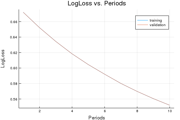
p1=plot(training_log_losses, label="training", title="LogLoss vs. Periods", ylabel="LogLoss", xlabel="Periods")
p1=plot!(validation_log_losses, label="validation")
println("Final LogLoss (on training data): ", training_log_losses[end])
# calculate additional ouputs
validation_probabilities = run(sess, y, Dict(feature_columns=> construct_feature_columns(validation_examples)));
return weight, bias, validation_probabilities, p1
end
weight, bias, validation_probabilities,  p1 = train_linear_classifier_model(
    0.0005, #learning rate
    1000, #steps
    50, #batch_size
    train_feature_mat,
    train_labels,
    test_features_mat,
    test_labels)
Training model...
LogLoss (on training data):
  period 1: 0.6721105081252955
  period 2: 0.6522005640636969
  period 3: 0.634401208607931
  period 4: 0.6183662540532432
  period 5: 0.6044376123838642
  period 6: 0.5920609187885028
  period 7: 0.5801279224633832
  period 8: 0.5697933602890288
  period 9: 0.5604221657436445
  period 10: 0.5519431087096996
Model training finished.
Final LogLoss (on training data): 0.5519431087096996


([-0.368462; 0.322629; … ; 0.125009; 0.192912], 0.03650506092723156, [0.585129; 0.387341; … ; 0.663437; 0.528799], Plot{Plots.GRBackend() n=2})
plot(p1)
The following function converts the validation probabilites back to 0-1-predictions.
# Function for converting probabilities to 0/1 decision
function castto01(probabilities)
    out=copy(probabilities)
    for i=1:length(probabilities)
        if(probabilities[i]<0.5)
            out[i]=0
        else
            out[i]=1
        end
    end
    return out
end
Let’s have a look at the accuracy of the model:
evaluation_metrics=DataFrame()
false_positive_rate, true_positive_rate, thresholds = sklm.roc_curve(
vec(construct_feature_columns(test_labels)), vec(validation_probabilities))
evaluation_metrics[:auc]=sklm.roc_auc_score(construct_feature_columns(test_labels), vec(validation_probabilities))
validation_predictions=castto01(validation_probabilities);
evaluation_metrics[:accuracy] = sklm.accuracy_score(collect(test_labels), validation_predictions)
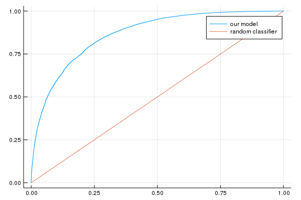
p2=plot(false_positive_rate, true_positive_rate, label="our model")
p2=plot!([0, 1], [0, 1], label="random classifier");
println("AUC on the validation set: ",  evaluation_metrics[:auc])
println("Accuracy on the validation set: ", evaluation_metrics[:accuracy])
AUC on the validation set: [0.865822]
Accuracy on the validation set: [0.781791]
plot(p2)
Task 2: Use a Deep Neural Network (DNN) Model
The above model is a linear model. It works quite well. But can we do better with a DNN model?
Let’s construct a NN classification model. Run the following cells, and see how you do.
function train_nn_classification_model(learning_rate,
steps,
batch_size,
hidden_units,
is_embedding,
keep_probability,
training_examples,
training_targets,
validation_examples,
validation_targets)
"""Trains a neural network classification model.
Args:
learning_rate: A `float`, the learning rate.
steps: A non-zero `int`, the total number of training steps. A training step
consists of a forward and backward pass using a single batch.
batch_size: A non-zero `int`, the batch size.
hidden_units: A vector describing the layout of the neural network.
is_embedding: 'true' or 'false' depending on if the first layer of the NN is an embedding layer.
keep_probability: A `float`, the probability of keeping a node active during one training step.
Returns:
p1: Plot of the loss function for the different periods.
y: The final layer of the TensorFlow network.
final_probabilities: Final predicted probabilities on the validation examples.
weight_export: The weights of the first layer of the NN
feature_columns: TensorFlow feature columns.
target_columns: TensorFlow target columns.
"""
periods = 10
steps_per_period = steps / periods
# Create feature columns.
feature_columns = placeholder(Float32, shape=[-1, size(training_examples,2)])
target_columns = placeholder(Float32, shape=[-1, size(training_targets,2)])
# Network parameters
push!(hidden_units,size(training_targets,2)) #create an output node that fits to the size of the targets
activation_functions = Vector{Function}(undef,size(hidden_units,1))
activation_functions[1:end-1] .= z->nn.dropout(nn.relu(z), keep_probability)
activation_functions[end] = nn.sigmoid #Last function should be idenity as we need the logits
# create network
flag=0
weight_export=Variable([1])
Zs = [feature_columns]
for (ii,(hlsize, actfun)) in enumerate(zip(hidden_units, activation_functions))
Wii = get_variable("W_$ii"*randstring(4), [get_shape(Zs[end], 2), hlsize], Float32)
bii = get_variable("b_$ii"*randstring(4), [hlsize], Float32)
if((is_embedding==true) & (flag==0))
Zii=Zs[end]*Wii
else
Zii = actfun(Zs[end]*Wii + bii)
end
push!(Zs, Zii)
if(flag==0)
weight_export=Wii
flag=1
end
end
y=Zs[end]
eps=1e-8
cross_entropy = -reduce_mean(log(y+eps).*target_columns + log(1-y+eps).*(1-target_columns))
features_batches, targets_batches = create_batches(training_examples, training_targets, steps, batch_size)
# Standard Adam Optimizer
my_optimizer=train.minimize(train.AdamOptimizer(learning_rate), cross_entropy)
run(sess, global_variables_initializer())
# Train the model, but do so inside a loop so that we can periodically assess
# loss metrics.
println("Training model...")
println("LogLoss error (on validation data):")
training_log_losses = []
validation_log_losses = []
for period in 1:periods
# Train the model, starting from the prior state.
for i=1:steps_per_period
features, labels = my_input_fn(features_batches, targets_batches, convert(Int,(period-1)*steps_per_period+i), batch_size)
run(sess, my_optimizer, Dict(feature_columns=>construct_feature_columns(features), target_columns=>construct_feature_columns(labels)))
end
# Take a break and compute log loss.
training_log_loss = run(sess, cross_entropy, Dict(feature_columns=> construct_feature_columns(training_examples), target_columns=>construct_feature_columns(training_targets)));
validation_log_loss = run(sess, cross_entropy, Dict(feature_columns=> construct_feature_columns(validation_examples), target_columns=>construct_feature_columns(validation_targets)));
# Occasionally print the current loss.
println(" period ", period, ": ", training_log_loss)
# Add the loss metrics from this period to our list.
push!(training_log_losses, training_log_loss)
push!(validation_log_losses, validation_log_loss)
end
println("Model training finished.")
# Calculate final predictions (not probabilities, as above).
final_probabilities = run(sess, y, Dict(feature_columns=> validation_examples, target_columns=>validation_targets))
final_predictions=0.0.*copy(final_probabilities)
final_predictions=castto01(final_probabilities)
accuracy = sklm.accuracy_score(collect(validation_targets), final_predictions)
println("Final accuracy (on validation data): ", accuracy)
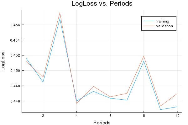
# Output a graph of loss metrics over periods.
p1=plot(training_log_losses, label="training", title="LogLoss vs. Periods", ylabel="LogLoss", xlabel="Periods")
p1=plot!(validation_log_losses, label="validation")
return p1, y, final_probabilities, weight_export, feature_columns, target_columns
end
sess=Session(Graph())
p1, y, final_probabilities, weight_export, feature_columns, target_columns = train_nn_classification_model(
    0.003, #learning rate
    1000, #steps
    50, #batch_size
    [20, 20], #hidden_units
    false, #is_embedding
    1.0, # keep probability
    train_feature_mat,
    train_labels,
    test_features_mat,
    test_labels)
Training model...
LogLoss error (on validation data):
  period 1: 0.4515786906010827
  period 2: 0.44849685369506703
  period 3: 0.45678289568993147
  period 4: 0.4460217305414473
  period 5: 0.4472715532609433
  period 6: 0.44637476140967014
  period 7: 0.4461147248181754
  period 8: 0.4512178549357173
  period 9: 0.44487838779238126
  period 10: 0.4452507003009877
Model training finished.
Final accuracy (on validation data): 0.7862314492579703


(Plot{Plots.GRBackend() n=2}, <Tensor Sigmoid:1 shape=(?, 1) dtype=Float32>, Float32[0.805678; 0.174846; … ; 0.918164; 0.58417], Variable{Float32}(<Tensor W_19xV4:1 shape=(50, 20) dtype=Float32>, <Tensor W_19xV4/Assign:1 shape=(50, 20) dtype=Float32>), <Tensor placeholder:1 shape=(?, 50) dtype=Float32>, <Tensor placeholder_2:1 shape=(?, 1) dtype=Float32>)
plot(p1)
evaluation_metrics=DataFrame()
false_positive_rate, true_positive_rate, thresholds = sklm.roc_curve(
    vec(construct_feature_columns(test_labels)), vec(final_probabilities))
evaluation_metrics[:auc]=sklm.roc_auc_score(construct_feature_columns(test_labels), vec(final_probabilities))
validation_predictions=castto01(final_probabilities);
evaluation_metrics[:accuracy]=accuracy = sklm.accuracy_score(collect(test_labels), validation_predictions)

p2=plot(false_positive_rate, true_positive_rate, label="our model")
p2=plot!([0, 1], [0, 1], label="random classifier");
println("AUC on the validation set: ",  evaluation_metrics[:auc])
println("Accuracy on the validation set: ", evaluation_metrics[:accuracy])
AUC on the validation set: [0.871958]
Accuracy on the validation set: [0.786231]
plot(p2)

Task 3: Use an Embedding with a DNN Model
In this task, we’ll implement our DNN model using an embedding column. An embedding column takes sparse data as input and returns a lower-dimensional dense vector as output. We’ll add the embedding layer as the first layer in the hidden_units-vector, and set is_embedding to true.
NOTE: In practice, we might project to dimensions higher than 2, like 50 or 100. But for now, 2 dimensions is easy to visualize.
sess=Session(Graph())
p1, y, final_probabilities, weight_export, feature_columns, target_columns = train_nn_classification_model(
    0.003, #learning rate
    1000, #steps
    50, #batch_size
    [2, 20, 20], #hidden_units
    true,
    1.0, # keep probability
    train_feature_mat,
    train_labels,
    test_features_mat,
    test_labels)
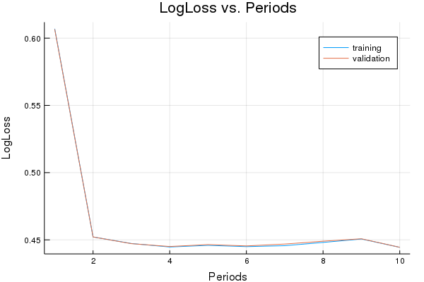
Training model...
LogLoss error (on validation data):
  period 1: 0.6069989732931624
  period 2: 0.4521562891019462
  period 3: 0.4472803943547435
  period 4: 0.44470490110825006
  period 5: 0.4459180835522875
  period 6: 0.4449739044671009
  period 7: 0.44566800024876874
  period 8: 0.4480791358543033
  period 9: 0.4506433883789002
  period 10: 0.4444382949975863
Model training finished.
Final accuracy (on validation data): 0.7886315452618105
plot(p1)
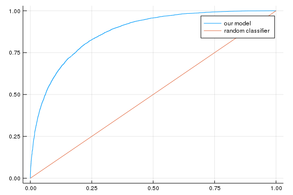
evaluation_metrics=DataFrame()
false_positive_rate, true_positive_rate, thresholds = sklm.roc_curve(
    vec(construct_feature_columns(test_labels)), vec(final_probabilities))
evaluation_metrics[:auc]=sklm.roc_auc_score(construct_feature_columns(test_labels), vec(final_probabilities))
validation_predictions=castto01(final_probabilities);
evaluation_metrics[:accuracy]=accuracy = sklm.accuracy_score(collect(test_labels), validation_predictions)

p2=plot(false_positive_rate, true_positive_rate, label="our model")
p2=plot!([0, 1], [0, 1], label="random classifier");
println("AUC on the validation set: ",  evaluation_metrics[:auc])
println("Accuracy on the validation set: ", evaluation_metrics[:accuracy])
AUC on the validation set: [0.873227]
Accuracy on the validation set: [0.788632]
plot(p2)
Task 4: Examine the Embedding
Let’s now take a look at the actual embedding space, and see where the terms end up in it. Do the following:
-
Run the following code to see the embedding we trained in Task 3. Do things end up where you’d expect?
-
Re-train the model by rerunning the code in Task 3, and then run the embedding visualization below again. What stays the same? What changes?
-
Finally, re-train the model again using only 10 steps (which will yield a terrible model). Run the embedding visualization below again. What do you see now, and why?
xy_coord=run(sess, weight_export, Dict(feature_columns=> test_features_mat, target_columns=>test_labels))
p3=plot(title="Embedding Space", xlims=(minimum(xy_coord[:,1])-0.3, maximum(xy_coord[:,1])+0.3),  ylims=(minimum(xy_coord[:,2])-0.1, maximum(xy_coord[:,2]) +0.3)  )
for term_index=1:length(informative_terms)
    p3=annotate!(xy_coord[term_index,1], xy_coord[term_index,1], informative_terms[term_index] )
end
plot(p3)
Task 5: Try to improve the model’s performance
See if you can refine the model to improve performance. A couple things you may want to try:
- Changing hyperparameters, or using a different optimizer than Adam (you may only gain one or two accuracy percentage points following these strategies).
- Adding additional terms to
informative_terms. There’s a full vocabulary file with all 30,716 terms for this data set that you can use at: https://storage.googleapis.com/mledu-datasets/sparse-data-embedding/terms.txt You can pick out additional terms from this vocabulary file, or use the whole thing.
In the following code, we will import the whole vocabulary file and run the model with it.
vocabulary=Array{String}(undef, 0)
open("terms.txt") do file
    for ln in eachline(file)
        push!(vocabulary, ln)
    end
end
vocabulary
30716-element Array{String,1}:
 "the"
 "."
 ","
 "and"
 "a"
 "of"
 "to"
 "is"
 "in"
 "i"
 "it"
 "this"
 "'"
 ⋮
 "soapbox"
 "softening"
 "user's"
 "od"
 "potter's"
 "renard"
 "impacting"
 "pong"
 "nobly"
 "nicol"
 "ff"
 "MISSING"
We will now load the test and training features matrices from disk. Open and run the Conversion of Movie-review data to one-hot encoding-notebook to prepare the IMDB_fullmatrix_datacolumns.jld-file. The notebook can be found here.
using JLD
train_features_full=load("IMDB_fullmatrix_datacolumns.jld", "train_features_full")
test_features_full=load("IMDB_fullmatrix_datacolumns.jld", "test_features_full")
Now run the session with the full vocabulary file. Again, this will take a long time to finish. It assigns about 50GB of memory.
sess=Session(Graph())
p1, y, final_probabilities, weight_export, feature_columns, target_columns = train_nn_classification_model(
    # TWEAK THESE VALUES TO SEE HOW MUCH YOU CAN IMPROVE THE RMSE
    0.003, #learning rate
    1000, #steps
    50, #batch_size
    [2, 20, 20], #hidden_units
    true,
    1.0, # keep probability
    train_features_full,
    train_labels,
    test_features_full,
    test_labels)
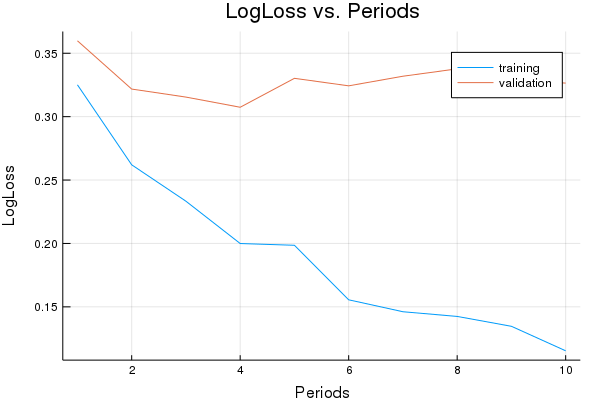
Training model...
LogLoss error (on validation data):
  period 1: 0.3251127531847735
  period 2: 0.26201559722924606
  period 3: 0.23330845378962484
  period 4: 0.19994648265169648
  period 5: 0.19856387267099854
  period 6: 0.15555357555980726
  period 7: 0.14615092534847945
  period 8: 0.1424473869184396
  period 9: 0.13466042909678566
  period 10: 0.11532863619817135
Model training finished.
Final accuracy (on validation data): 0.8650346013840554
plot(p1)
evaluation_metrics=DataFrame()
false_positive_rate, true_positive_rate, thresholds = sklm.roc_curve(
vec(construct_feature_columns(test_labels)), vec(final_probabilities))
evaluation_metrics[:auc]=sklm.roc_auc_score(construct_feature_columns(test_labels), vec(final_probabilities))
validation_predictions=castto01(final_probabilities);
evaluation_metrics[:accuracy]=accuracy = sklm.accuracy_score(collect(test_labels), validation_predictions)
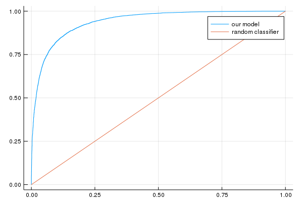
p2=plot(false_positive_rate, true_positive_rate, label="our model")
p2=plot!([0, 1], [0, 1], label="random classifier");
println("AUC on the validation set: ", evaluation_metrics[:auc])
println("Accuracy on the validation set: ", evaluation_metrics[:accuracy])
AUC on the validation set: [0.940777]
Accuracy on the validation set: [0.865035]
plot(p2)
Task 6: Try out sparse matrices
We will now convert the feature matrices from the previous step to sparse matrices and re-run our code. The sparse matrices take about 350MB of memory. The code for the NN will still convert the sparse matrix containing the data for the current batch to a full matrix, which leads to a memory requirement of about 35GB.
train_features_sparse=sparse(train_features_full)
test_features_sparse=sparse(test_features_full)
# For saving the data
#save("IMDB_sparsematrix_datacolumns.jld", "train_features_sparse", train_features_sparse, "test_features_sparse", test_features_sparse)
sess=Session(Graph())
p1, y, final_probabilities, weight_export, feature_columns, target_columns = train_nn_classification_model(
    0.003, #learning rate
    1000, #steps
    50, #batch_size
    [2, 20, 20], #hidden_units
    true,
    1.0, # keep probability
    train_features_sparse,
    train_labels,
    test_features_sparse,
    test_labels)
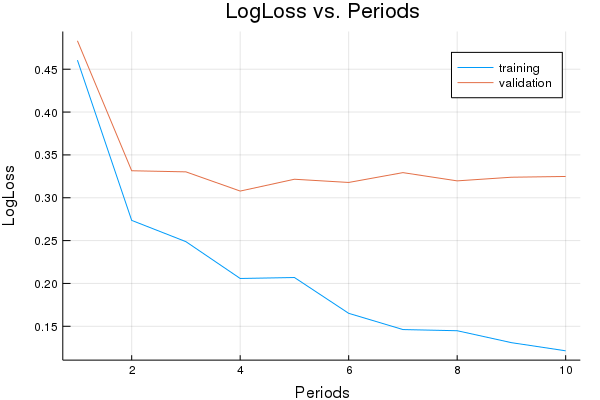
Training model...
LogLoss error (on validation data):
  period 1: 0.4605575853814918
  period 2: 0.27356117272016794
  period 3: 0.2487382422782251
  period 4: 0.2057872125802281
  period 5: 0.20691236441998723
  period 6: 0.16511000500632206
  period 7: 0.1461716377437531
  period 8: 0.14480918371448573
  period 9: 0.13087959631432583
  period 10: 0.12136018625662037
Model training finished.
Final accuracy (on validation data): 0.8677547101884076
plot(p1)
evaluation_metrics=DataFrame()
false_positive_rate, true_positive_rate, thresholds = sklm.roc_curve(
    vec(construct_feature_columns(test_labels)), vec(final_probabilities))
evaluation_metrics[:auc]=sklm.roc_auc_score(construct_feature_columns(test_labels), vec(final_probabilities))
validation_predictions=castto01(final_probabilities);
evaluation_metrics[:accuracy]=accuracy = sklm.accuracy_score(collect(test_labels), validation_predictions)

p2=plot(false_positive_rate, true_positive_rate, label="our model")
p2=plot!([0, 1], [0, 1], label="random classifier");
println("AUC on the validation set: ",  evaluation_metrics[:auc])
println("Accuracy on the validation set: ", evaluation_metrics[:accuracy])
AUC on the validation set: [0.941214]
Accuracy on the validation set: [0.867755]
plot(p2)

A Final Word
We may have gotten a DNN solution with an embedding that was better than our original linear model, but the linear model was also pretty good and was quite a bit faster to train. Linear models train more quickly because they do not have nearly as many parameters to update or layers to backprop through.
In some applications, the speed of linear models may be a game changer, or linear models may be perfectly sufficient from a quality standpoint. In other areas, the additional model complexity and capacity provided by DNNs might be more important. When defining your model architecture, remember to explore your problem sufficiently so that you know which space you’re in.