In this second part, we create a synthetic feature and remove some outliers from the data set.
The Jupyter notebook can be downloaded here.
This notebook is based on the file Synthetic Features and Outliers, which is part of Google’s Machine Learning Crash Course.
# Licensed under the Apache License, Version 2.0 (the "License");
# you may not use this file except in compliance with the License.
# You may obtain a copy of the License at
#
# https://www.apache.org/licenses/LICENSE-2.0
#
# Unless required by applicable law or agreed to in writing, software
# distributed under the License is distributed on an "AS IS" BASIS,
# WITHOUT WARRANTIES OR CONDITIONS OF ANY KIND, either express or implied.
# See the License for the specific language governing permissions and
# limitations under the License.
Synthetic Features and Outliers
Learning Objectives:
- Create a synthetic feature that is the ratio of two other features
- Use this new feature as an input to a linear regression model
- Improve the effectiveness of the model by identifying and clipping (removing) outliers out of the input data
Let’s revisit our model from the previous First Steps with TensorFlow exercise.
First, we’ll import the California housing data into DataFrame:
Setup
using Plots
gr(fmt=:png)
using DataFrames
using TensorFlow
import CSV
using Random
using Statistics

sess=Session()

california_housing_dataframe = CSV.read("california_housing_train.csv", delim=",");
california_housing_dataframe[:median_house_value] /= 1000.0
california_housing_dataframe
| longitude | latitude | housing_median_age | total_rooms | total_bedrooms | population | households | median_income | median_house_value | |
|---|---|---|---|---|---|---|---|---|---|
| Float64⍰ | Float64⍰ | Float64⍰ | Float64⍰ | Float64⍰ | Float64⍰ | Float64⍰ | Float64⍰ | Float64 | |
| 1 | -114.31 | 34.19 | 15.0 | 5612.0 | 1283.0 | 1015.0 | 472.0 | 1.4936 | 66.9 |
| 2 | -114.47 | 34.4 | 19.0 | 7650.0 | 1901.0 | 1129.0 | 463.0 | 1.82 | 80.1 |
| 3 | -114.56 | 33.69 | 17.0 | 720.0 | 174.0 | 333.0 | 117.0 | 1.6509 | 85.7 |
| 4 | -114.57 | 33.64 | 14.0 | 1501.0 | 337.0 | 515.0 | 226.0 | 3.1917 | 73.4 |
| 5 | -114.57 | 33.57 | 20.0 | 1454.0 | 326.0 | 624.0 | 262.0 | 1.925 | 65.5 |
| 6 | -114.58 | 33.63 | 29.0 | 1387.0 | 236.0 | 671.0 | 239.0 | 3.3438 | 74.0 |
| 7 | -114.58 | 33.61 | 25.0 | 2907.0 | 680.0 | 1841.0 | 633.0 | 2.6768 | 82.4 |
| 8 | -114.59 | 34.83 | 41.0 | 812.0 | 168.0 | 375.0 | 158.0 | 1.7083 | 48.5 |
| 9 | -114.59 | 33.61 | 34.0 | 4789.0 | 1175.0 | 3134.0 | 1056.0 | 2.1782 | 58.4 |
| 10 | -114.6 | 34.83 | 46.0 | 1497.0 | 309.0 | 787.0 | 271.0 | 2.1908 | 48.1 |
| 11 | -114.6 | 33.62 | 16.0 | 3741.0 | 801.0 | 2434.0 | 824.0 | 2.6797 | 86.5 |
| 12 | -114.6 | 33.6 | 21.0 | 1988.0 | 483.0 | 1182.0 | 437.0 | 1.625 | 62.0 |
| 13 | -114.61 | 34.84 | 48.0 | 1291.0 | 248.0 | 580.0 | 211.0 | 2.1571 | 48.6 |
| 14 | -114.61 | 34.83 | 31.0 | 2478.0 | 464.0 | 1346.0 | 479.0 | 3.212 | 70.4 |
| 15 | -114.63 | 32.76 | 15.0 | 1448.0 | 378.0 | 949.0 | 300.0 | 0.8585 | 45.0 |
| 16 | -114.65 | 34.89 | 17.0 | 2556.0 | 587.0 | 1005.0 | 401.0 | 1.6991 | 69.1 |
| 17 | -114.65 | 33.6 | 28.0 | 1678.0 | 322.0 | 666.0 | 256.0 | 2.9653 | 94.9 |
| 18 | -114.65 | 32.79 | 21.0 | 44.0 | 33.0 | 64.0 | 27.0 | 0.8571 | 25.0 |
| 19 | -114.66 | 32.74 | 17.0 | 1388.0 | 386.0 | 775.0 | 320.0 | 1.2049 | 44.0 |
| 20 | -114.67 | 33.92 | 17.0 | 97.0 | 24.0 | 29.0 | 15.0 | 1.2656 | 27.5 |
| 21 | -114.68 | 33.49 | 20.0 | 1491.0 | 360.0 | 1135.0 | 303.0 | 1.6395 | 44.4 |
| 22 | -114.73 | 33.43 | 24.0 | 796.0 | 243.0 | 227.0 | 139.0 | 0.8964 | 59.2 |
| 23 | -114.94 | 34.55 | 20.0 | 350.0 | 95.0 | 119.0 | 58.0 | 1.625 | 50.0 |
| 24 | -114.98 | 33.82 | 15.0 | 644.0 | 129.0 | 137.0 | 52.0 | 3.2097 | 71.3 |
| 25 | -115.22 | 33.54 | 18.0 | 1706.0 | 397.0 | 3424.0 | 283.0 | 1.625 | 53.5 |
| 26 | -115.32 | 32.82 | 34.0 | 591.0 | 139.0 | 327.0 | 89.0 | 3.6528 | 100.0 |
| 27 | -115.37 | 32.82 | 30.0 | 1602.0 | 322.0 | 1130.0 | 335.0 | 3.5735 | 71.1 |
| 28 | -115.37 | 32.82 | 14.0 | 1276.0 | 270.0 | 867.0 | 261.0 | 1.9375 | 80.9 |
| 29 | -115.37 | 32.81 | 32.0 | 741.0 | 191.0 | 623.0 | 169.0 | 1.7604 | 68.6 |
| 30 | -115.37 | 32.81 | 23.0 | 1458.0 | 294.0 | 866.0 | 275.0 | 2.3594 | 74.3 |
| ⋮ | ⋮ | ⋮ | ⋮ | ⋮ | ⋮ | ⋮ | ⋮ | ⋮ | ⋮ |
Next, we’ll set up our input functions, and define the function for model training:
function create_batches(features, targets, steps, batch_size=5, num_epochs=0)

    if(num_epochs==0)
        num_epochs=ceil(batch_size*steps/length(features))
    end

    features_batches=Union{Float64, Missings.Missing}[]
    target_batches=Union{Float64, Missings.Missing}[]

    for i=1:num_epochs

        select=shuffle(1:length(features))

        append!(features_batches, features[select])
        append!(target_batches, targets[select])
    end

    return features_batches, target_batches
end
function next_batch(features_batches, targets_batches, batch_size, iter)

    select=mod((iter-1)*batch_size+1, length(features_batches)):mod(iter*batch_size, length(features_batches));

    ds=features_batches[select];
    target=targets_batches[select];

    return ds, target
end
function my_input_fn(features_batches, targets_batches, iter, batch_size=5, shuffle_flag=1)
    """Trains a linear regression model of one feature.

    Args:
      features: DataFrame of features
      targets: DataFrame of targets
      batch_size: Size of batches to be passed to the model
      shuffle: True or False. Whether to shuffle the data.
      num_epochs: Number of epochs for which data should be repeated. None = repeat indefinitely
    Returns:
      Tuple of (features, labels) for next data batch
    """

    # Construct a dataset, and configure batching/repeating.
    ds, target = next_batch(features_batches, targets_batches, batch_size, iter)

    # Shuffle the data, if specified.
    if shuffle_flag==1
      select=Random.shuffle(1:size(ds, 1));
        ds = ds[select,:]
        target = target[select, :]
    end

    # Return the next batch of data.
    return convert(Matrix{Float64},ds), convert(Matrix{Float64},target)
end
function train_model(learning_rate, steps, batch_size, input_feature=:total_rooms)
  """Trains a linear regression model of one feature.

  Args:
    learning_rate: A `float`, the learning rate.
    steps: A non-zero `int`, the total number of training steps. A training step
      consists of a forward and backward pass using a single batch.
    batch_size: A non-zero `int`, the batch size.
    input_feature: A `symbol` specifying a column from `california_housing_dataframe`
      to use as input feature.
  """

  periods = 10
  steps_per_period = steps / periods

  my_feature = input_feature
  my_feature_data = convert.(Float32,california_housing_dataframe[my_feature])
  my_label = :median_house_value
  targets = convert.(Float32,california_housing_dataframe[my_label])

  # Create feature columns.
  feature_columns = placeholder(Float32)
  target_columns = placeholder(Float32)

  # Create a linear regressor object.
  m=Variable(0.0)
  b=Variable(0.0)
  y=m.*feature_columns .+ b
  loss=reduce_sum((target_columns - y).^2)
  run(sess, global_variables_initializer())
  features_batches, targets_batches = create_batches(my_feature_data, targets, steps, batch_size)

  # Use gradient descent as the optimizer for training the model.
  #my_optimizer=train.minimize(train.GradientDescentOptimizer(learning_rate), loss)
  my_optimizer=(train.GradientDescentOptimizer(learning_rate))
  gvs = train.compute_gradients(my_optimizer, loss)
  capped_gvs = [(clip_by_norm(grad, 5.), var) for (grad, var) in gvs]
  my_optimizer = train.apply_gradients(my_optimizer,capped_gvs)

  # Set up to plot the state of our model's line each period.
  sample = california_housing_dataframe[rand(1:size(california_housing_dataframe,1), 300),:];
  p1=scatter(sample[my_feature], sample[my_label], title="Learned Line by Period", ylabel=my_label, xlabel=my_feature,color=:coolwarm)
  colors= [ColorGradient(:coolwarm)[i] for i in range(0,stop=1, length=periods+1)]

  # Train the model, but do so inside a loop so that we can periodically assess
  # loss metrics.
  println("Training model...")
  println("RMSE (on training data):")
  root_mean_squared_errors = []
  for period in 1:periods
    # Train the model, starting from the prior state.
   for i=1:steps_per_period
    features, labels = my_input_fn(features_batches, targets_batches, convert(Int,(period-1)*steps_per_period+i), batch_size)
    run(sess, my_optimizer, Dict(feature_columns=>features, target_columns=>labels))
   end
    # Take a break and compute predictions.
    predictions = run(sess, y, Dict(feature_columns=> my_feature_data));

    # Compute loss.
    mean_squared_error = mean((predictions- targets).^2)
    root_mean_squared_error = sqrt(mean_squared_error)
    # Occasionally print the current loss.
    println("  period ", period, ": ", root_mean_squared_error)
    # Add the loss metrics from this period to our list.
    push!(root_mean_squared_errors, root_mean_squared_error)
    # Finally, track the weights and biases over time.

    # Apply some math to ensure that the data and line are plotted neatly.
    y_extents = [0 maximum(sample[my_label])]
    weight = run(sess,m)
    bias = run(sess,b)
    x_extents = (y_extents .- bias) / weight
    x_extents = max.(min.(x_extents, maximum(sample[my_feature])),
                           minimum(sample[my_feature]))
    y_extents = weight .* x_extents .+ bias
    p1=plot!(x_extents', y_extents', color=colors[period], linewidth=2)
 end

  predictions = run(sess, y, Dict(feature_columns=> my_feature_data));
  weight = run(sess,m)
  bias = run(sess,b)

  println("Model training finished.")

  # Output a graph of loss metrics over periods.
  p2=plot(root_mean_squared_errors, title="Root Mean Squared Error vs. Periods", ylabel="RMSE", xlabel="Periods")

  # Output a table with calibration data.
  calibration_data = DataFrame()
  calibration_data[:predictions] = predictions
  calibration_data[:targets] = targets
  describe(calibration_data)

  println("Final RMSE (on training data): ", root_mean_squared_errors[end])
  println("Final Weight (on training data): ", weight)
  println("Final Bias (on training data): ", bias)

  return p1, p2, calibration_data
end
Task 1: Try a Synthetic Feature
Both the total_rooms and population features count totals for a given city block.
But what if one city block were more densely populated than another? We can explore how block density relates to median house value by creating a synthetic feature that’s a ratio of total_rooms and population.
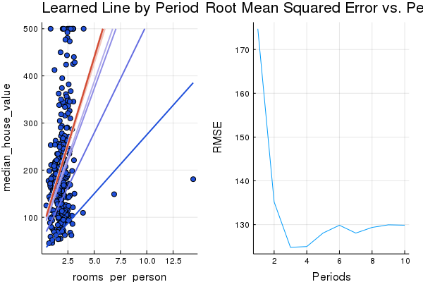
In the cell below, we create a feature called rooms_per_person, and use that as the input_feature to train_model().
california_housing_dataframe[:rooms_per_person] =(
    california_housing_dataframe[:total_rooms] ./ california_housing_dataframe[:population]);
p1, p2, calibration_data= train_model(
    0.05, # learning rate
    1000, # steps
    5, # batch size
    :rooms_per_person #feature
)
Training model...
RMSE (on training data):
  period 1: 174.73499015754794
  period 2: 135.18378014936647
  period 3: 124.81483763650894
  period 4: 124.99348861666715
  period 5: 128.0855648925441
  period 6: 129.86065434272652
  period 7: 128.06995380520772
  period 8: 129.3628149624267
  period 9: 129.9533622545398
  period 10: 129.8691255721607
Model training finished.
Final RMSE (on training data): 129.8691255721607
Final Weight (on training data): 74.18756812501896
Final Bias (on training data): 67.78876122300292
plot(p1, p2, layout=(1,2), legend=false)
Task 2: Identify Outliers
We can visualize the performance of our model by creating a scatter plot of predictions vs. target values. Ideally, these would lie on a perfectly correlated diagonal line.
We use scatter to create a scatter plot of predictions vs. targets, using the rooms-per-person model you trained in Task 1.
Do you see any oddities? Trace these back to the source data by looking at the distribution of values in rooms_per_person.
scatter(calibration_data[:predictions], calibration_data[:targets], legend=false)
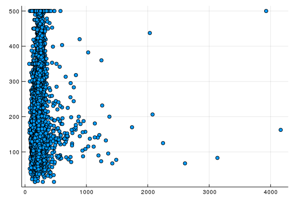
The calibration data shows most scatter points aligned to a line. The line is almost vertical, but we’ll come back to that later. Right now let’s focus on the ones that deviate from the line. We notice that they are relatively few in number.
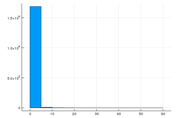
If we plot a histogram of rooms_per_person, we find that we have a few outliers in our input data:
histogram(california_housing_dataframe[:rooms_per_person], nbins=20, legend=false)
Task 3: Clip Outliers
We see if we can further improve the model fit by setting the outlier values of rooms_per_person to some reasonable minimum or maximum.
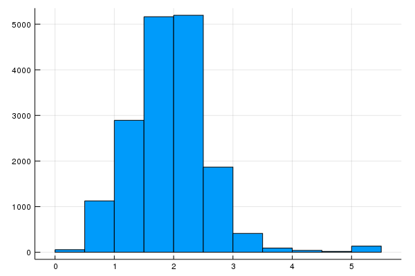
The histogram we created in Task 2 shows that the majority of values are less than 5. Let’s clip rooms_per_person to 5, and plot a histogram to double-check the results.
california_housing_dataframe[:rooms_per_person] = min.(
    california_housing_dataframe[:rooms_per_person],5)

histogram(california_housing_dataframe[:rooms_per_person], nbins=20, legend=false)
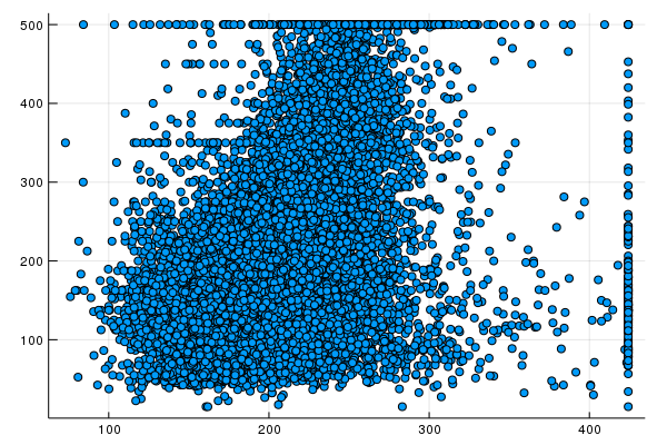
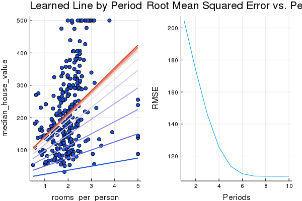
To verify that clipping worked, let’s train again and print the calibration data once more:
p1, p2, calibration_data= train_model(
    0.05, # learning rate
    500, # steps
    10, # batch size
    :rooms_per_person #feature
)
Training model...
RMSE (on training data):
  period 1: 204.65393150901195
  period 2: 173.7183427312223
  period 3: 145.97809305428905
  period 4: 125.39350453104828
  period 5: 113.5851230428793
  period 6: 108.94376856469054
  period 7: 107.51132608903492
  period 8: 107.37501891367756
  period 9: 107.35720127223883
  period 10: 107.36959825293329
Model training finished.
Final RMSE (on training data): 107.36959825293329
Final Weight (on training data): 70.5
Final Bias (on training data): 71.72122192382814
plot(p1, p2, layout=(1,2), legend=false)
scatter(calibration_data[:predictions], calibration_data[:targets], legend=false)